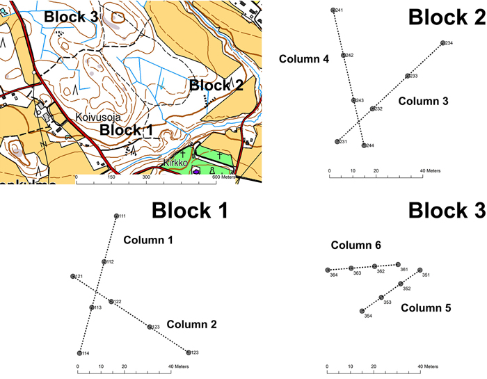
Fig. 1. Layout of the Block – Column -sample point design at the Jokioinen site (Blocks 1–3).
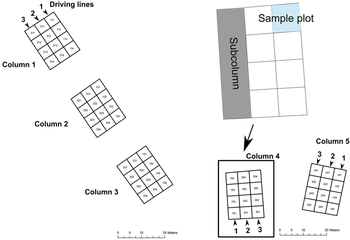
Fig. 2. Layout of the Block – Column – Sub-column -sample plot design at the Vihti site (Block 4 and 5).
| Table 1. The main stand characteristics of the test sites. | |||||
| DBH | Height | Volume | |||
| Forest site | Block | Mean, cm | Mean, m | m3 ha–1 | |
| Modelling data | |||||
| Jokioinen | 1 | Pine | 28.3 | 25.9 | 178 |
| Spruce | 27.6 | 24.8 | 185 | ||
| Birch | 8.4 | 7.4 | 17 | ||
| Total | 27.8 | 25.1 | 391 | ||
| Jokioinen | 2 | Pine | 20.2 | 16.8 | 37 |
| Spruce | 22.6 | 21.1 | 193 | ||
| Birch | 24.6 | 22.1 | 112 | ||
| Total | 23.6 | 21.6 | 351 | ||
| Jokioinen | 3 | Pine | 12.4 | 13.1 | 59 |
| Spruce | 11.4 | 12.7 | 49 | ||
| Birch | 10.8 | 13.1 | 86 | ||
| Total | 11.4 | 13.2 | 195 | ||
| Test data | |||||
| Vihti | 4 | Pine | - | - | - |
| Spruce | 12.7 | 14.5 | 262 | ||
| Birch | - | - | - | ||
| Total | 12.7 | 14.5 | 262 | ||
| Vihti | 5 | Pine | - | - | - |
| Spruce | 15.8 | 15.4 | 220 | ||
| Birch | 17.6 | 16.0 | 108 | ||
| Total | 17.0 | 15.8 | 328 | ||
| Table 2. Mean (and standard deviation in parenthesis) of bulk density (BD), organic content (%), clay content (%) of the mineral soil samples and the thickness of humus layer (cm) in the modelling data set and test data set. N = Number of measurements. | ||||||
| Block | Column | BD g cm–3 | Organic content % | Clay % | Humus layer cm | N |
| Modelling data | ||||||
| 1 | 1.0 | 1.33 (0.07) | 3.5 (1.0) | 5.1 (1.6) | 4 | 4 |
| 2.0 | 1.18 (0.09) | 4.3 (0.8) | 6.5 (1.8) | 4 | 4 | |
| 2 | 3.0 | 0.97 (0.08) | 9.5 (1.3) | 34.6 (3.1) | 2 | 4 |
| 4.0 | 0.91 (0.24) | 11.9 (2.8) | 37.0 (8.3) | 3 | 4 | |
| 3 | 5.0 | 1.14 (0.20) | 7.9 (1.8) | 52.4 (5.5) | 8 | 4 |
| 6.0 | 1.32 (0.20) | 5.7 (2.0) | 43.4 (14.9) | 12 | 4 | |
| All | 1.14 (0.22) | 7.1 (3.4) | 29.8 (19.4) | 5.6 (4.1) | 24 | |
| Test data | ||||||
| 4 | 1.0 | 0.92 (0.13) | 9.7 (1.2) | 50.6 (3.8) | 4 | 12 |
| 2.0 | 0.88 (0.18) | 9.4 (1.2) | 51.3 (2.4) | 3 | 12 | |
| 3.0 | 0.99 (0.07) | 8.5 (0.8) | 44.1 (2.6) | 4 | 12 | |
| 5 | 4.0 | 1.13 (0.11) | 8.3 (2.0) | 22.5 (9.2) | 5 | 12 |
| 5.0 | 1.26 (0.15) | 8.0 (3.1) | 40.5 (13.1) | 11 | 12 | |
| All | 1.03 (0.2) | 8.4 (2.4) | 40.4 (15.3) | 5.2 (3.5) | 84 | |
| Table 3. Mean, standard deviation, minimum and maximum values for PR010ms, PR015ms and VWC by block in the Jokioinen data. | ||||
| Block | PR010ms MPa | PR015ms MPa | VWC % | |
| 1 | Mean | 0.848 | 0.956 | 22.8 |
| Std. Deviation | 0.262 | 0.299 | 5.7 | |
| Minimum | 0.470 | 0.542 | 14.6 | |
| Maximum | 1.542 | 1.640 | 40.0 | |
| 2 | Mean | 1.153 | 1.616 | 31.6 |
| Std. Deviation | 0.525 | 0.789 | 8.6 | |
| Minimum | 0.324 | 0.381 | 18.5 | |
| Maximum | 2.891 | 4.190 | 49.8 | |
| 3 | Mean | 1.536 | 1.746 | 36.9 |
| Std. Deviation | 0.593 | 0.617 | 7.5 | |
| Minimum | 0.536 | 0.733 | 19.2 | |
| Maximum | 3.491 | 3.294 | 50.9 | |
| Total | Mean | 1.179 | 1.439 | 30.4 |
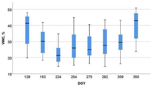
Fig. 3. Box-plot illustration of the VWC by day of the year (DOY). The bottom and top of the box are upper and lower quartiles, and the bolded black line indicates the median, lowest and highest point of the vector minimum and maximum values.
| Table 4. Mean, standard deviation, minimum and maximum values for PR010, PR015 and VWC by block in the Vihti data. | ||||
| Block | PR015 MPa | PR020 MPa | VWC % | |
| 4 | Mean | 1.072 | 1.249 | 33.6 |
| Std. Deviation | 0.365 | 0.436 | 8.0 | |
| Minimum | 0.572 | 0.670 | 18.4 | |
| Maximum | 2.296 | 2.588 | 45.3 | |
| 5 | Mean | 0.875 | 1.138 | 39.6 |
| Std. Deviation | 0.153 | 0.212 | 6.6 | |
| Minimum | 0.677 | 0.786 | 26.3 | |
| Maximum | 1.150 | 1.523 | 51.4 | |
| Total | Mean | 1.028 | 1.224 | 34.9 |
| Sampling was not possible in block 5 on the last testing occasion (December) | ||||
| Table 5. Mixed regression models predicting PR of the first 10 cm (InvPR = Inverse of PR) of the inorganic soil. | ||||||||
| Model | Model 1 | Model 2 | Model 3 | Model 4 | ||||
| Dependent variable | InvPR010ms | InvPR010ms | InvPR010ms | InvPR010ms | ||||
| Parameter | Estimate (SE) | Sig. | Estimate (SE) | Sig. | Estimate (SE) | Sig. | Estimate (SE) | Sig. |
| Fixed | ||||||||
| Intercept | 0.165 (0.368) | .668 | 0.670 (0.282) | .022 | –0.314 (0.288) | .434 | –0.290 (0.135) | .034 |
| VWC | 0.0336 (0.00289) | .000 | 0.0325 (0.00292) | .000 | 0.0340 (0.00289) | .000 | 0.0333 (0.00292) | .000 |
| BD | –0.446 (0.272) | .114 | –0.912 (0.249) | .001 | - | - | ||
| Three clay classes | ||||||||
| Clay class 1 (<10%) | 0.885 (0.173) | .250 | 0.971 (0.122) | .000 | 0.795 (0.465) | .335 | 0.786 (0.142) | .000 |
| Clay class 2 (10–30%) | 0.340 (0.180) | .074 | 0.506 (0.198) | .019 | 0.179 (0.161) | .281 | 0.175 (0.235) | .464 |
| Clay class 3 (>30%) | 0 | 0 | 0 | 0 | ||||
| ui | 0.0080 (0.125) | .522 | - | 0.138 (0.203) | .678 | - | ||
| vij | 0.0279 (0.0136) | .041 | 0.0417 (0.0184) | .023 | 0.0335 (0.0149) | .024 | 0.0850 (0.0309) | .006 |
| σ2meas | 0.0908 (0.0105) | .000 | 0.0924 (0.0108) | .000 | 0.0897 (0.0103) | .000 | 0.0900 (0.0104) | .000 |
| ρmeas | 0.0267 (0.101) | .791 | 0.0378 (0.102) | .711 | 0.0211 (0.100) | .833 | 0.0280 (0.102) | .784 |
| AIC | 139.1 | 143.3 | 140.7 | 151.6 | ||||
| Table 6. Mixed regression models predicting PR of the first 15 cm (InvPR = Inverse of PR) of the inorganic soil. | ||||||||
| Model | Model 5 | Model 6 | Model 7 | Model 8 | ||||
| Dependent variable | InvPR015ms | InvPR015ms | InvPR015 | InvPR015 | ||||
| Parameter | Estimate (SE) | Sig. | Estimate (SE) | Sig. | Estimate (SE) | Sig. | Estimate (SE) | Sig. |
| Fixed | ||||||||
| Intercept | 0.276 (0.270) | .331 | 0.457 (0.259) | .052 | –0.242 (0.178) | .323 | –0.220 (0.106) | .040 |
| VWC | 0.0263 (0.00238) | .000 | 0.0259 (0.00237) | .000 | 0.0267 (0.00238) | .000 | 0.0261 (0.00239) | .000 |
| BD | –0.483 (0.228) | .049 | –0.643 (0.198) | 003 | - | - | ||
| Three clay classes | ||||||||
| Clay class 1 (<10%) | 0.852 (0.167) | .134 | 0.881 (0.0975) | .000 | 0.754 (0.270) | .213 | 0.746 (0.106) | .000 |
| Clay class 2 (10–30%) | 0.303 (0.160) | .072 | 0.360 (0.158) | .033 | 0.128 (0.146) | .392 | 0.126 (0.174) | .480 |
| Clay class 3 (>30%) | 0 | 0 | 0 | 0 | ||||
| ui | 0.0122 (0.0268) | .648 | - | 0.0431 (0.0678) | .636 | - | ||
| vij | 0.0237 (0.0110) | .031 | 0.0253 (0.0115) | .028 | 0.0287 (0.0123) | .019 | 0.0443 (0.0171) | .010 |
| σ2meas | 0.0594 (0.00716) | .000 | 0.0597 (0.0724) | .000 | 0.0588 (0.00705) | .000 | 0.0591 (0.00716) | .000 |
| ρmeas | 0.0929 (0.103) | .371 | 0.0971 (0.104) | .352 | 0.0902 (0.104) | .383 | 0.0978 (0.105) | .350 |
| AIC | 58.7 | 57.4 | 61.0 | 64.2 | ||||
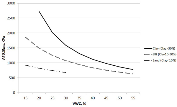
Fig. 4. The PR of the soil for the first 15 cm below the surface of the inorganic soil (model 5 from Table 6) by VWC and clay content (BD constant 0.9 g cm–3).
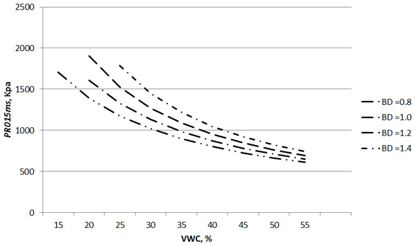
Fig. 5. The PR of the soil for the first 15 cm below the surface of the inorganic soil (model 5 from Table 6) by VWC and BD (Clay class 3).
| Table 7. Accuracy of the PR models in terms of bias and mean absolute error (MAE). Error is a result of the predicted value subtracted with the measured value. | ||||||||
| Variable | Models utilized | Predictors | Bias | 95% confidence interval for Bias | MAE | |||
| kPa | % | kPa | kPa | % | ||||
| PR0est15 | Model 1 and Model 9 | Clay class (2 or 3), VWC and BD | –59 | –5.9 | –130 | 11 | 191 | 19.1 |
| PRest015 | Model 3 and Model 5 | Clay class (2 or 3) and VWC | –0.1 | –0.01 | –88 | 88 | 220 | 22.0 |
| PRest020 | Model 5 and Model 10 | Clay class (2 or 3), VWC and BD | 11 | 1.0 | –70 | 93 | 225 | 18.8 |
| PRest020 | Model 7 and Model 10 | Clay class (2 or 3) and VWC | 115 | 9.6 | –2 | 232 | 286 | 23.9 |
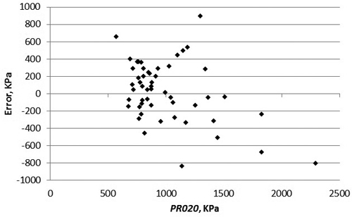
Fig. 6. Residuals of the predictions of the PR of first 20 cm above the ground surface constructed with models 5 and 10. Error is a result of the predicted value subtracted with the measured value.