| Table 1. The average stand characteristics calculated from harvester STM data. The given volumes do not contain the saw log reduction. | ||||||||
| Stand | Species | N ha–1 | G m2 ha–1 | DG cm | HG m | Logs m3 ha–1 | Pulp m3 ha–1 | Size l |
| 1 | Pine | 374.67 | 20.87 | 27.55 | 23.43 | 167.94 | 24.94 | 584 |
| Spruce | 14.67 | 0.41 | 22.30 | 18.48 | 2.09 | 1,10 | 245 | |
| Birch | 21.33 | 0.43 | 19.63 | 17.81 | 1.35 | 1.72 | 161 | |
| 2 | Pine | 227.27 | 17.26 | 32.39 | 28.94 | 186.10 | 19.93 | 904 |
| Spruce | 13.64 | 0.57 | 27.95 | 22.12 | 4.55 | 1.23 | 422 | |
| Birch | 23.64 | 0.58 | 22.94 | 17.76 | 2.14 | 2.28 | 190 | |
| 3 | Pine | 296.25 | 17.65 | 28.68 | 23.81 | 164.89 | 22.61 | 631 |
| Spruce | 109.38 | 3.42 | 24.61 | 18.66 | 19.07 | 10.47 | 269 | |
| Birch | 90.00 | 2.05 | 23.75 | 20.20 | 10.13 | 7.60 | 201 | |
| 4 | Pine | 234.29 | 22.05 | 37.07 | 30.18 | 246.73 | 22.23 | 1141 |
| Spruce | 668.57 | 31.61 | 30.77 | 26.11 | 314.20 | 71.21 | 573 | |
| Birch | 50.00 | 2.64 | 31.79 | 26.46 | 23.06 | 6.32 | 590 | |
| 5 | Pine | 140.00 | 12.12 | 34.50 | 28.17 | 130.53 | 11.75 | 1013 |
| Spruce | 223.13 | 9.23 | 28.72 | 23.82 | 83.67 | 19.30 | 460 | |
| Birch | 51.25 | 3.55 | 35.44 | 27.32 | 34.22 | 5.42 | 776 | |
| 6 | Pine | 251.43 | 18.74 | 32.03 | 27.53 | 198.69 | 20.33 | 863 |
| Spruce | 494.29 | 28.85 | 30.26 | 26.09 | 301.37 | 55.73 | 721 | |
| Birch | 88.57 | 1.17 | 16.41 | 17.58 | 2.59 | 6.18 | 104 | |
| 7 | Pine | 157.43 | 10.26 | 31.09 | 23.06 | 95.51 | 10.84 | 666 |
| Spruce | 225.25 | 5.13 | 24.69 | 19.30 | 30.72 | 15.02 | 199 | |
| Birch | 75.74 | 2.02 | 28.37 | 22.36 | 13.40 | 5.26 | 249 | |
| Average | 182.42 | 10.03 | 28.14 | 23.29 | 96.81 | 16.26 | 522 | |
| N denotes the number of stems, G is the basal area, DG is the basal area-weighted mean diameter, HG is Lorey’s height, Logs is the saw log volume, Pulp is the pulpwood volume, and Size is the average stem size of merchantable wood. | ||||||||
| Table 2. Assortment volume (m3) estimates and the number (N) of cut trees for the clear-cut sections based on the 41 timber trade contracts and the actual harvested characteristic by tree species. The estimated number of cut trees was given by dividing the sum of the pulpwood and the saw logs for the contracts, with the average stem size given in m3. The average difference (contract – harvested) and the standard deviations between these characteristics are given in the last 3 lines. | ||||||
| Pine | Spruce | Birch | ||||
| Variable | Mean | Std | Mean | Std | Mean | Std |
| Pulpwood, contracts | 70.6 | 65.1 | 66.0 | 63.4 | 37.0 | 64.7 |
| Pulpwood, harvested | 67.3 | 82.1 | 64.9 | 57.1 | 59.4 | 76.6 |
| Saw logs, contracts | 138.0 | 137.5 | 158.8 | 191.2 | 4.7 | 8.0 |
| Saw logs, harvested | 139.8 | 114.9 | 140.0 | 170.0 | 3.3 | 5.5 |
| N of cut trees, contracts | 461.1 | 407.2 | 421.5 | 440.5 | 195.3 | 284.9 |
| N of cut trees, harvested | 668.0 | 780.2 | 707.1 | 683.2 | 503.6 | 604.4 |
| Difference between contract and actual harvested characteristics | ||||||
| Pulpwood | 3.3 | 55.5 | 1.1 | 32.1 | –22.4 | 43.1 |
| Saw logs | –1.8 | 87.0 | 18.9 | 67.4 | 1.4 | 9.3 |
| Number of cut trees | –206.9 | 660.1 | –285.6 | 404.3 | –308.3 | 419.3 |
| Table 3. Prediction errors in stand characteristics when the truncated Weibull distribution was solved using optimization for the modelling data set (STM based input data). | |||||||
| Stand | Species | Iterations | G m2 ha–1 | DG cm | HG m | Saw logs m3 ha–1 | Pulpwood m3 ha–1 |
| 1 | Pine | 118 | 2.55 | 0.53 | –0.05 | 0.00 | 0.00 |
| Spruce | 35 | –0.07 | –2.14 | 2.93 | 0.01 | –0.05 | |
| Birch | 36 | –0.07 | –2.96 | 3.22 | –0.01 | –0.02 | |
| 2 | Pine | 33 | –0.97 | –2.81 | 2.54 | 0.05 | 1.38 |
| Spruce | 39 | –0.19 | –1.89 | 4.19 | 0.00 | 0.02 | |
| Birch | 58 | –0.09 | –0.80 | 2.30 | 0.01 | 0.02 | |
| 3 | Pine | 118 | 0.04 | 0.79 | –0.20 | 0.02 | –0.68 |
| Spruce | 29 | –0.35 | 0.01 | 0.96 | –0.10 | 0.18 | |
| Birch | 40 | –0.35 | –1.22 | 1.83 | 0.08 | –0.35 | |
| 4 | Pine | 39 | –0.30 | –0.59 | 0.39 | –0.01 | –0.42 |
| Spruce | 31 | –2.67 | –1.84 | 0.14 | 1.20 | –1.35 | |
| Birch | 29 | –0.09 | 3.25 | 1.81 | 0.03 | 0.40 | |
| 5 | Pine | 32 | –0.45 | –2.74 | 1.45 | –0.01 | 0.36 |
| Spruce | 25 | –2.08 | –2.62 | 1.71 | –1.06 | –2.49 | |
| Birch | 101 | –0.19 | 2.28 | 1.76 | 0.00 | 0.00 | |
| 6 | Pine | 32 | –0.34 | –1.56 | –0.23 | –0.09 | –2.26 |
| Spruce | 34 | –2.36 | –1.66 | 0.67 | 0.02 | 0.81 | |
| Birch | 36 | –0.19 | –1.54 | 1.38 | 0.03 | –0.20 | |
| 7 | Pine | 1000 | –0.07 | 1.96 | 0.20 | 0.00 | 0.00 |
| Spruce | 37 | –1.02 | –1.38 | 0.91 | 0.26 | –1.42 | |
| Birch | 27 | –0.49 | 0.57 | 3.25 | 0.82 | –1.70 | |
| Bias | –0.46 | –0.78 | 1.48 | 0.06 | –0.37 | ||
| Bias% | –4.63 | –2.77 | 6.37 | 0.06 | –2.28 | ||
| St. dev | 1.05 | 1.77 | 1.26 | 0.40 | 0.97 | ||
| G denotes the basal area, DG is the basal area-weighted mean diameter, and HG is Lorey’s height. | |||||||
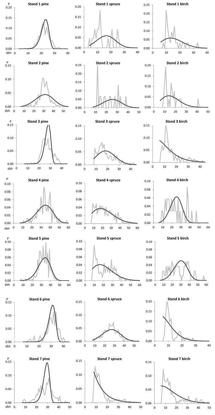
Fig. 1. The observed (grey line) and predicted (black line) species-specific breast height diameter (dbh) distributions for the modelling data set of seven clear-cut stands.
| Table 4. Parameters b and c for the optimized Weibull distribution and the Kolmogorov-Smirnov (KS) goodness-of-fit statistics, i.e., supremum S, critical KS test value and KS-quotient by Tham (1988), for each distribution in the modelling data set. The restricted distributions (KS-q > 1.0) at the 0.1 significance level are shown in bold. | ||||||
| Stand | Species | b | c | S | KS test | KS-q |
| 1 | Pine | 27.65652 | 10.75086 | 0.0744 | 0.0516 | 1.4229 |
| Spruce | 22.84091 | 3.42576 | 0.1337 | 0.2609 | 0.5065 | |
| Birch | 17.08886 | 2.04147 | 0.1625 | 0.2164 | 0.7519 | |
| 2 | Pine | 33.85908 | 3.93423 | 0.0611 | 0.0774 | 0.7885 |
| Spruce | 28.18846 | 3.58795 | 0.2532 | 0.3160 | 0.7931 | |
| Birch | 18.15757 | 2.07353 | 0.1396 | 0.2400 | 0.5927 | |
| 3 | Pine | 28.54391 | 11.99995 | 0.0945 | 0.0562 | 1.5388 |
| Spruce | 21.48926 | 2.72832 | 0.0361 | 0.0925 | 0.4363 | |
| Birch | 14.6169 | 1.48271 | 0.0908 | 0.1020 | 0.8490 | |
| 4 | Pine | 36.92752 | 4.46618 | 0.0467 | 0.0956 | 0.4740 |
| Spruce | 24.96678 | 1.98449 | 0.0213 | 0.0566 | 0.8099 | |
| Birch | 28.00898 | 4.50419 | 0.0729 | 0.2069 | 0.3601 | |
| 5 | Pine | 35.85537 | 3.9325 | 0.0570 | 0.0818 | 0.5271 |
| Spruce | 25.53413 | 2.2826 | 0.0643 | 0.0648 | 0.8973 | |
| Birch | 32.39969 | 4.36577 | 0.0510 | 0.1352 | 0.8471 | |
| 6 | Pine | 32.92287 | 4.46401 | 0.0658 | 0.0923 | 0.7783 |
| Spruce | 29.96348 | 3.48296 | 0.0280 | 0.0658 | 0.3697 | |
| Birch | 9.88933 | 1.44835 | 0.1242 | 0.1554 | 0.7981 | |
| 7 | Pine | 29.8171 | 11.9427 | 0.0941 | 0.0686 | 0.9683 |
| Spruce | 13.22079 | 1.29523 | 0.0527 | 0.0574 | 0.6641 | |
| Birch | 17.06155 | 1.52872 | 0.0691 | 0.0989 | 0.6441 | |
| Table 5. The difference (m3 for the clear-cut section) between the input assortment volumes from timber trade contracts and that of the output from the solved truncated Weibull distribution by tree species without saw log reduction and with the optional saw log reductions: MELA96, MELA05 and Bucking simulator (Malinen et al. 2007). The best results are shown in bold. | ||||||||
| Reduction: | Without | MELA96 | MELA05 | Bucking simulator | ||||
| Assortment: | Pulpwood | Saw logs | Pulpwood | Saw logs | Pulpwood | Saw logs | Pulpwood | Saw logs |
| Pine | 40.11 | 2.6 | 10.85 | 1.19 | 1.2 | 0.12 | 10.14 | 1.15 |
| Spruce | 43.49 | 2.27 | 39.96 | 2.16 | 7.86 | 0.63 | 32.26 | 1.81 |
| Birch | 6.65 | 0.32 | 4.39 | 0.58 | 4.39 | 0.54 | 3.46 | 0.53 |
| Total | 30.27 | 1.53 | 18.51 | 1.31 | 4.48 | 0.43 | 14.78 | 1.11 |
| Table 6. The average goodness-of-fit tests according to the Kolmogorov-Smirnov quotient (KS-q) by Tham (1988) and the Error Index (EI) by Reynolds et al. (1988). Tests are given by tree species and total with the given saw log reduction option. The number of rejected cases (KS-q > 1) by tree species with the used saw log reduction percentage (slr%) in addition to the total number of rejected cases. The best results are shown in bold. | ||||||||
| Reduction | Without | MELA96 | MELA05 | Bucking simulator | ||||
| Test | KS-q | EI | KS-q | EI | KS-q | EI | KS-q | EI |
| Pine | 1.0755 | 0.5567 | 1.2637 | 0.6794 | 1.3584 | 0.7126 | 1.2687 | 0.6756 |
| Spruce | 1.5596 | 0.8457 | 1.5628 | 0.8344 | 1.3334 | 0.7500 | 1.5415 | 0.8287 |
| Birch | 1.5626 | 0.9844 | 1.4631 | 0.9062 | 1.4614 | 0.9080 | 1.4207 | 0.8771 |
| Total | 1.3903 | 0.7914 | 1.4226 | 0.8040 | 1.3787 | 0.7880 | 1.4034 | 0.7912 |
| KS test: | rejected | (slr%) | rejected | (slr%) | rejected | (slr%) | rejected | (sl%) |
| Pine | 12/41 | (0) | 18/41 | (16) | 20/41 | (24) | 19/41 | (18) |
| Spruce | 28/40 | (0) | 28/40 | (2) | 24/40 | (18) | 29/40 | (6) |
| Birch | 29/40 | (0) | 21/40 | (30) | 21/40 | (29) | 19/40 | (41) |
| Total | 69/121 | 67/121 | 65/121 | 67/121 | ||||
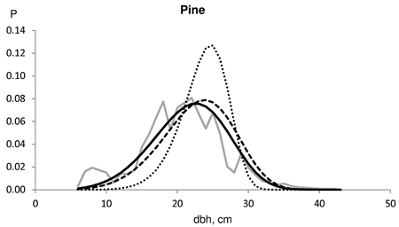
Fig. 2. Example of the harvested dbh distributions for Scots pine in test data (solid grey line). The number of harvested trees (N) and assortment volumes for a clear-cut section of 2.3 ha for the contract/harvester data were: N 1020/930; pulpwood 130/65 m3; saw logs 280/234 m3. The Kolmogorov-Smirnov quotient for the predicted distribution was 0.7719 without saw log reduction (solid line), 1.0738 using 16% MELA96 reduction (broken line) and 1.7620 using 24% MELA05 reduction (dotted line).
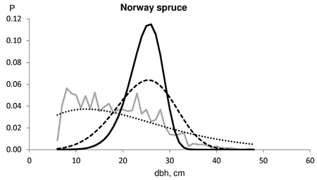
Fig. 3. Example of the harvested dbh distributions for Norway spruce in test data (solid grey line). The number of harvested trees (N) and assortment volumes for a clear-cut section of 2.7 ha for the contract/harvester data were: N 704/1102; pulpwood 100/74 m3; saw logs 255/302 m3. The Kolmogorov-Smirnov quotient for the predicted distribution was 2.608 without saw log reduction (solid line), 1.577 using 6% Bucking simulator-reduction (broken line) and 0.6777 with 18% MELA05 reduction (dotted line).
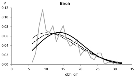
Fig. 4. Example of the harvested dbh distributions for birch in test data (solid grey line). The number of harvested trees (N) and the assortment volumes for a clear-cut section of 4.6 ha for the contract/harvester data were: N 533/207; pulpwood 70/30 m3; saw logs 10/2 m3. The Kolmogorov-Smirnov quotient for the predicted distribution was 0.766 without saw log reduction (solid line), 0.657 using 30% MELA96 reduction (broken line) and 0.600 with 41% Bucking simulator-reduction (dotted line).