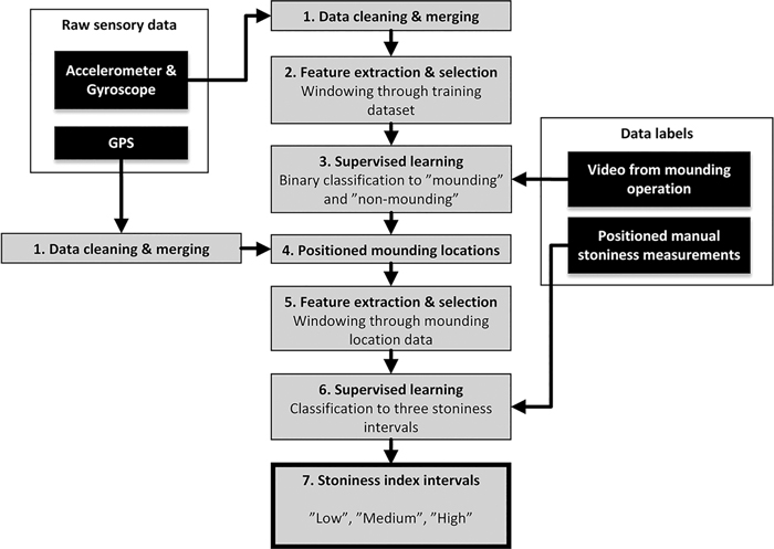
Fig. 1. Stoniness classification process of forest soil, based on the excavator IMU data.
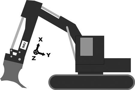
Fig. 2. A drawing of the measurement setup and the coordinate axes in the excavator. The location of the measurement device is marked with the “IMU” label (IMU = inertial measurement unit).
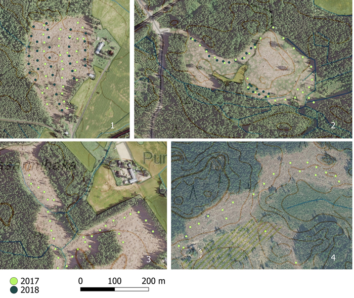
Fig. 3. Manual stoniness measurements at four different sites. The circles are the center points for the series of 10 bar insertions and the color indicates the year of the measurements. (Aerial photo © National Land Survey of Finland 2018).
| Table 1. Initial features before feature selection. | ||
| Features for IMU signals | ||
| Basic descriptive statistics | Mean | Minimum |
| Median | Maximum | |
| Standard deviation (STD) | 25th percentile | |
| Variance | 75th percentile | |
| Median absolute deviation (MAD) | Skewness | |
| Interquartile range (IQR) | Kurtosis | |
| Signal metrics | Peak to peak | |
| Root-mean-square level (RMS) | ||
| Signal power | ||
| 1-lag autocorrelation | ||
| Frequency domain properties | Dominant frequency | |
| Dominant frequency magnitude | ||
| Correlations | Correlation coefficients between axes | |
| Table 2. Features ranked highest by the ReliefF algorithm. | ||
| Ranked features for each axis by the ReliefF algorithm (Rank order) | ||
| Activity recognition | Stoniness classification | |
| Accelerometer X | - | Minimum (10) Maximum (18) Peak to peak (20) Dominant frequency magnitude (21) Autocorrelation (22) |
| Accelerometer Y | Kurtosis (4) Maximum (5) MAD (11) IQR (14) 75-percentile (24) | Max (2) Peak to peak (3) Autocorrelation (5) 75-percentile (12) STD (14) Minimum (16) Dominant frequency (23) Power (24) Variance (25) |
| Accelerometer Z | Dominant frequency magnitude (7) Autocorrelation (12) Mean (15) 75-percentile (22) Median (25) | Autocorrelation (13) MAD (15) IQR (19) |
| Gyroscope X | MAD (1) Dominant frequency magnitude (10) 75-percentile (21) | Autocorrelation (6) |
| Gyroscope Y | - | Autocorrelation (8) |
| Gyroscope Z | Minimum (3) 75-percentile (6) Median (8) 25-percentile (13) Mean (20) MAD (23) | - |
| Correlation coeff. | Acc. X – Acc. Y (2) Acc. Y – Acc. Z (9) Gyro. Y – Gyro. Z (19) | Gyro. X – Gyro. Y (1) Acc. Z – Gyro. Y (4) Acc. X – Acc. Y (7) Acc. Y – Gyro. X (9) Acc. Z – Gyro. X (11) Acc. X – Gyro. Z (17) |
| STD = standard deviation, MAD = Median absolute deviation, IQR = Interquartile range. | ||
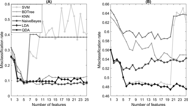
Fig. 4. The misclassification rate with an increasing number of features selected by the ReliefF algorithm in (A) activity recognition and (B) stoniness classification.
| Table 3. Selected features in activity recognition by the SFS algorithm. | ||||||
| Selected features for each axis by the SFS algorithm (activity recognition) | ||||||
| SVM | BDTree | KNN | NaïveBayes | LDA | QDA | |
| Accelerometer X | RMS Peak to peak | Minimum | - | - | - | - |
| Accelerometer Y | Variance | STD | Maximum STD Peak to peak | STD | Variance | Variance |
| Accelerometer Z | - | - | - | - | - | - |
| Gyroscope X | - | - | 25-percentile | Median | MAD | MAD |
| Gyroscope Y | - | Peak to peak | - | - | - | - |
| Gyroscope Z | - | - | - | Mean | Mean | Mean |
| SVM = Support Vector Machine, BDTree = Binary Decision Tree, KNN = K-Nearest Neighbors, LDA = Linear Discriminant Analysis, QDA = Quadratic Discriminant Analysis. RMS = Root-mean-square level, STD = standard deviation, MAD = Median absolute deviation. | ||||||
| Table 4. Selected features in stoniness classification by the SFS algorithm. | ||||||
| Selected features for each axis by the SFS algorithm (stoniness classification) | ||||||
| SVM | BDTree | KNN | NaïveBayes | LDA | QDA | |
| Accelerometer X | Dom. freq. | - | - | - | RMS 75-percentile Dom. freq. mag. | RMS 75-percentile Dom. freq. mag. |
| Accelerometer Y | Autocorrelation | - | - | Mean Skewness Autocorrelation | Median Maximum Variance Power Autocorrelation | Median Maximum Variance Power Autocorrelation |
| Accelerometer Z | STD 75-percentile | - | - | Median 75-percentile | Mean | Mean |
| Gyroscope X | Maximum | - | - | - | Maximum Peak to peak | Maximum Peak to peak |
| Gyroscope Y | Maximum | - | - | MAD | MAD Kurtosis Peak to peak | MAD Kurtosis Peak to peak |
| Gyroscope Z | Minimum | Dom. freq. | Dom. freq. | - | Minimum Autocorrelation | Minimum Autocorrelation |
| Correlation coeff. | - | - | - | Acc. X – Acc. Y Acc. X – Gyro. Y | Acc. X – Gyro. Y | Acc. X – Gyro. Y |
| SVM = Support Vector Machine, BDTree = Binary Decision Tree, KNN = K-Nearest Neighbors, LDA = Linear Discriminant Analysis, QDA = Quadratic Discriminant Analysis. RMS = Root-mean-square level, STD = standard deviation, MAD = Median absolute deviation. | ||||||
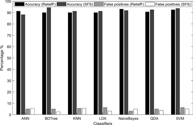
Fig. 5. The accuracy and percentage of false-positive predictions in the activity recognition using two feature-selection algorithms, ReliefF and Sequential Feature Selection (SFS).
| Table 5. The stoniness prediction accuracy. | |||||||
| Stoniness prediction accuracy (%) | |||||||
| SVM | BDTree | KNN | NaïveBayes | LDA | QDA | ANN | |
| Point prediction (ReliefF) | 43.3 | 43.8 | 42.6 | 42.6 | 47.6 | 44.6 | 43.0 |
| Point prediction (SFS) | 45.0 | 37.7 | 45.6 | 44.6 | 44.6 | 40.8 | 43.0 |
| Grid prediction (ReliefF) | 66.1 | 69.6 | 37.5 | 64.3 | 35.7 | 57.1 | 62.5 |
| Grid prediction (SFS) | 75.0 | 26.8 | 46.4 | 50.0 | 28.6 | 53.6 | 62.5 |
| SVM = Support Vector Machine, BDTree = Binary Decision Tree, KNN = K-Nearest Neighbors, LDA = Linear Discriminant Analysis, QDA = Quadratic Discriminant Analysis, ANN = a neural network model. | |||||||
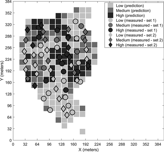
Fig. 6. Predicted stoniness classes and manual measurements for the first site.
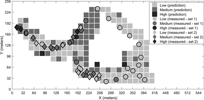
Fig. 7. Predicted stoniness classes and manual measurements for the second site.
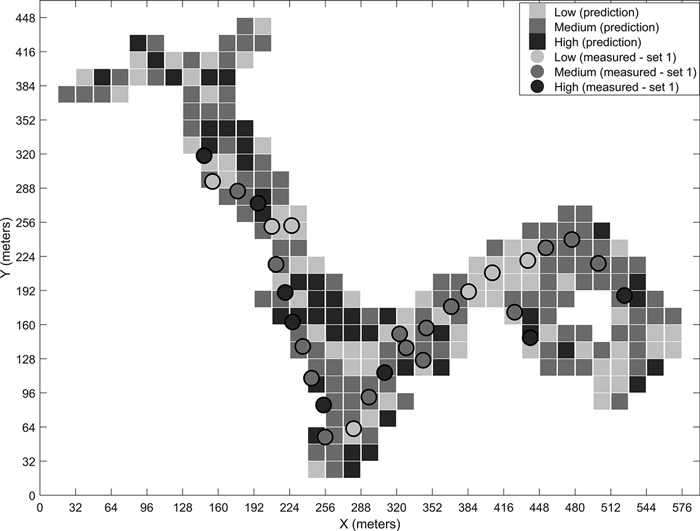
Fig. 8. Predicted stoniness classes and manual measurements for the third site.
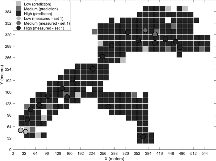
Fig. 9. Predicted stoniness classes and manual measurements for the fourth site.
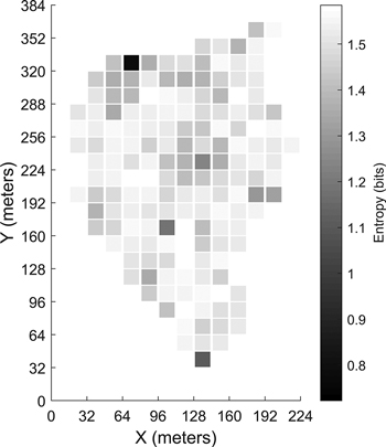
Fig. 10. Entropy calculated for each grid cell in the first site.