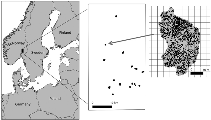
Fig. 1. Location of the study area (left), the distribution of the harvested stands within the study area (middle) and layout of grid cells (harvester plots) within the clear-cut polygon (right). Each harvested stand (middle) or tree (right) is marked with a black dot.
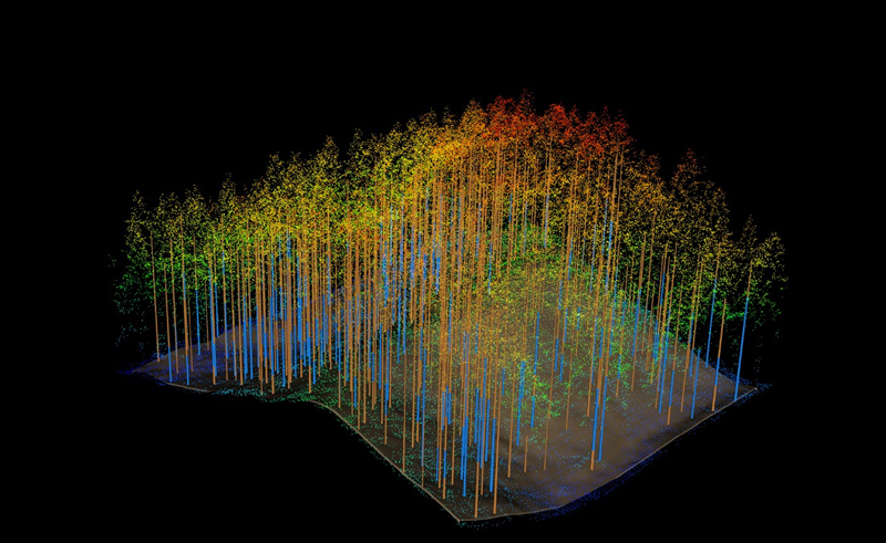
Fig. 2. Example of recorded tree positions along with tree sizes as measured by the harvester and with the three-dimensional point cloud of ALS data for a single stand. The blue and brown colors for the tree stems represent sawn wood and pulpwood, respectively.
| Table 1. Mean values (standard deviations in brackets) of the considered attributes at harvester plot and stand level using different harvester plot sizes. | |||||||||
| Plot size (m2) | n | VTotal, m3 ha–1 | VSpruce, m3 ha–1 | VPine, m3 ha–1 | VDeciduous, m3 ha–1 | GTotal, m2 ha–1 | NTotal, ha–1 | VSawSpruce, m3 ha–1 | DmeanSpruce, cm |
| Harvester plot | |||||||||
| 200 | 2306 | 299.0 (138.2) | 260.9 (138.7) | 21.2 (57.5) | 17.0 (38.9) | 27.5 (13.0) | 781 (349.1) | 235.4 (135.6) | 21.9 (4.0) |
| 400 | 949 | 275.1 (115.1) | 242.4 (117.3) | 18.1 (46.9) | 14.7 (30.1) | 25.4 (11.0) | 711 (294.4) | 219.2 (113.7) | 21.9 (3.5) |
| 900 | 285 | 290.8 (90.4) | 258.9 (96.9) | 17.5 (42.9) | 14.5 (27.2) | 27.1 (9.0) | 742.7 (230.3) | 235.0 (94.3) | 21.9 (2.8) |
| 1600 | 99 | 300.0 (66.3) | 272.8 (77.2) | 13.3 (35.5) | 13.9 (21.7) | 28.5 (7.5) | 753.3 (185.9) | 249.3 (75.3) | 22.1 (2.3) |
| Stand | |||||||||
| 200 | 47 | 298.3 (97.7) | 259.3 (103.1) | 17.3 (37.0) | 21.8 (30.8) | 27.6 (8.7) | 808 (222.0) | 232.7 (105.5) | 21.3 (2.8) |
| 400 | 38 | 245.3 (80.8) | 213.6 (84.1) | 19.1 (39.3) | 12.6 (16.1) | 22.6 (7.4) | 660 (211.5) | 190.1 (83.0) | 21.2 (2.9) |
| 900 | 24 | 266.5 (64.9) | 231.4 (67.3) | 24.1 (39.4) | 11.0 (13.1) | 24.6 (6.0) | 733 (148.4) | 203.4 (72.8) | 20.7 (2.6) |
| 1600 | 15 | 281.2 (53.8) | 241.0 (66.1) | 29.8 (48.7) | 10.4 (14.4) | 24.7 (6.4) | 699 (141.5) | 217.1 (63.9) | 21.1 (2.0) |
| VTotal is total merchantable volume and VSpruce, VPine and VDeciduous are merchantable volumes for species Norway spruce, Scots pine and deciduous species, respectively. GTotal and NTotal are basal area and number of stems of the whole living tree stock, respectively. VsawSpruce and DmeanSpruce are merchantable volume of the sawn timber part of the stem diameter distribution and mean diameter of the Norway spruce, respectively. | |||||||||
| Table 2. Description of the metrics derived from the height distribution of the ALS data for individual harvester plots. The metrics were calculated separately for the two respective sets of first return and last return echoes. All metrics where calculated using only the canopy echoes (height > 2 m), with the exception of the density metrics where the total number of echoes also included echoes with height < 2 m. | |
| Metric | Description |
| Hmean | Mean canopy echo height. |
| Hsd | Standard deviation of the canopy echo height distribution. |
| Hcv | Coefficient of variance for the canopy echo height distribution. |
| Hkurt | Kurtosis of the canopy echo height distribution. |
| Hskewness | Skewness of the canopy echo height distribution. |
| H10,, ..., H90 | The 10th, 20th, ..., 90th percentile of the of the canopy echo heights. |
| d0, d1, …, d10 | Density metrics: The height range between the lowest canopy echo and the 95% percentile was divided into 10 fractions of equal length and metrics were computed as the number of echoes above each fraction divided by the total number of echoes (including echoes with height < 2 m). |
| Table 3. Estimation errors indicated by RMSE% (RMSE values in brackets) of different total and species-specific stand attributes with different harvester plot sizes. | ||||
| Plot size 200 m2 | Plot size 400 m2 | Plot size 900 m2 | Plot size 1600 m2 | |
| Number of stands | 19 | 18 | 14 | 8 |
| VTotal , m3 ha–1 | 8.4 (25.5) | 9.5 (26.0) | 11.6 (32.9) | 11.9 (35.2) |
| NTotal, ha–1 | 19.3 (144.9) | 17.8 (123.0) | 16.3 (116.2) | 14.3 (104.6) |
| GTotal, m2 ha–1 | 9.1 (2.9) | 9.8 (2.8) | 12.5 (3.7) | 13.0 (4.0) |
| VSpruce, m3 ha–1 | 18.9 (47.7) | 18.96 (46.0) | 22.5 (57.6) | 19.1 (52.2) |
| VPine, m3 ha–1 | 140.1 (33.5) | 169.2 (33.1) | 237.4 (41.1) | 193.1 (21.8) |
| VDeciduous, m3 ha–1 | 85.4 (12.4) | 96.7 (12.5) | 140.8 (15.1) | 136.4 (16.9) |
| VsawSpruce, m3 ha–1 | 20.3 (49.0) | 22.0 (48.5) | 26.2 (61.1) | 22.3 (55.9) |
| DmeanSpruce, cm | 10.6 (2.3) | 11.0 (2.4) | 12.0 (2.6) | 9.7 (2.2) |
| D20, cm | 14.0 (2.0) | 15.2 (2.2) | 18.3 (2.7) | 16.8 (2.5) |
| D40, cm | 12.7 (2.4) | 13.2 (2.5) | 15.7 (3.0) | 12.8 (2.5) |
| D60, cm | 11.3 (2.6) | 11.5 (2.7) | 12.7 (3.0) | 10.4 (2.5) |
| D80, cm | 10.3 (2.8) | 10.3 (2.9) | 10.0 (2.8) | 8.8 (2.5) |
| Error Index (mean value) | 0.15 | 0.17 | 0.18 | 0.18 |
| D20, D40, D60 and D80 are cumulative diameter percentiles of 20%, 40%, 60% and 80% of the number of stems, respectively. For other abbreviations, see Table 1. | ||||
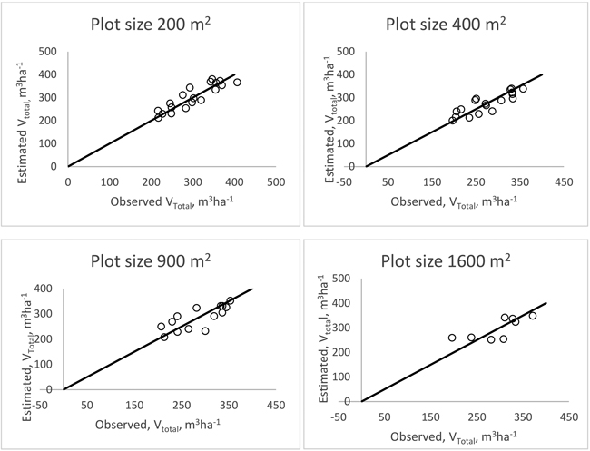
Fig. 3. Merchantable volume estimation validation at stand level using different plot sizes.
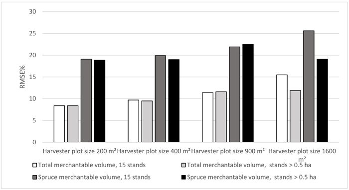
Fig. 4. Estimation errors of total merchantable volume and spruce merchantable volume when the same stands (n = 15) were used in the validation across all harvester plot sizes. Also results from the validation using stands larger than 0.5 hectares are shown for comparison.
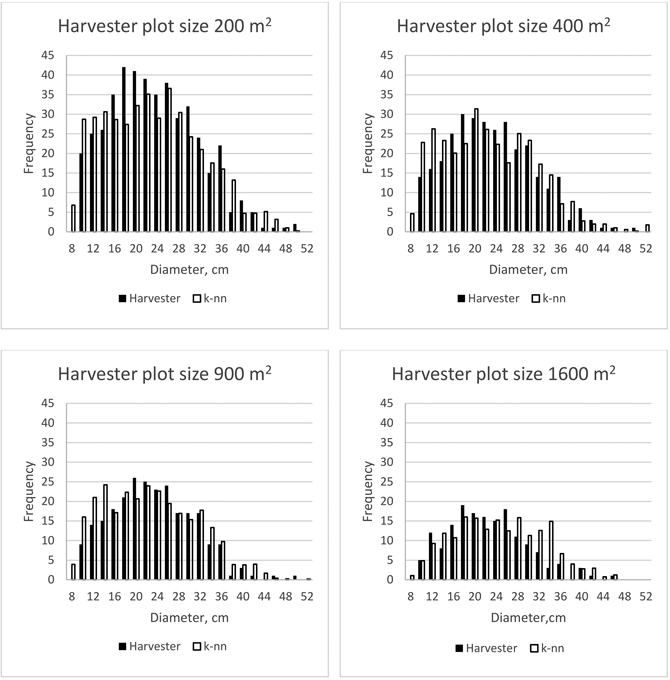
Fig. 5. Example of stand-level stem diameter distributions based on harvester measurements and k-nn based estimation using different harvester plot sizes.
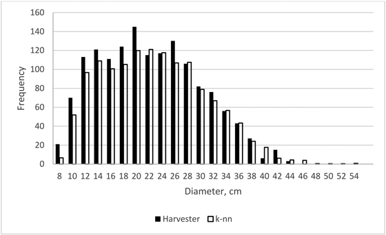
Fig. 6. Stem-level diameter distribution estimate of the smallest error index value (0.05) in the case of plot size 200 m2.
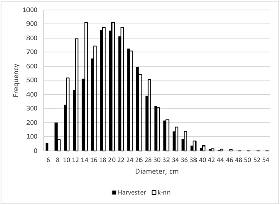
Fig. 7. Stem-level diameter distribution estimate of the largest error index value (0.22) in the case of plot size 200 m2.