| Table 1. Applied quality requirements for Scots pine sawlog. |
| Crookedness, curves | - Max. 1 cm within 1 m distance |
| Technical defects (e.g. scar) | - Allowed outside log cylinder |
| Min. length | 37 dm |
| Min. diameter | 15 cm |
| Max. diameter of branches: | |
| - Dead/dry | 4 cm |
| - Living | 6 cm |
| Not allowed: | - Curves on multiple directions |
| - Decay |
| - Blue stain -fungi infection |
| - Insect holes |
| - Cracks |
| - Internal items |
| Table 2. The distribution of quality assessed Scots pines by site type index. Calculated with all pines and different subsets of pines. Relative proportions in parentheses. The mean and the standard deviation of the observed relative sawlog reduction are also shown. The study area is located in boreal forest in eastern Finland. |
| All | OMT | MT | VT |
| All pines | 1235 | 46 | 787 | 402 |
| Flawless pines | 346 (28.0%) | 4 (8.6%) | 211 (26.8%) | 131 (32.6%) |
| Partly defective pines | 625 (50.6%) | 21 (45.7%) | 406 (51.6%) | 198 (49.3%) |
| Fully defective pines | 264 (21.4%) | 21 (45.7%) | 170 (21.6%) | 73 (18.1%) |
| MeanSR | 39.8 | 64.1 | 40.1 | 36.4 |
| SdSR | 36.9 | 37.8 | 37.0 | 35.6 |
| Table 3. Main characteristics of the studied plots (15 × 15 m, n = 164) and stands (30 × 30 m, n = 41). Stand-level values are shown in parentheses. The study area is located in boreal forest in eastern Finland. |
| | Min | Max | Mean | Sd |
| Theoretical sawlog V (m3 ha–1) | 13.7 (21.0) | 742.8 (557.3) | 175.1 (175.1) | 129.7 (121.2) |
| Factual sawlog V (m3 ha–1) | 0 (8) | 631.9 (519.0) | 124.3 (124.3) | 105.6 (100.0) |
| Pine prop. of the theoretical sawlog V (%) | 8.8 (42.5) | 100.0 (100.0) | 84.5 (84.6) | 23.4 (18.8) |
| Pine prop. of the factual sawlog V (%) | 0 (28.6) | 100.0 (100.0) | 79.4 (78.8) | 28.9 (24.3) |
| Mean dbh (cm) | 10.9 (12.0) | 35.5 (28.8) | 18.0 (17.6) | 4.7 (4.1) |
| Mean h (m) | 9.7 (10.8) | 31.3 (25.6) | 16.3 (16.1) | 3.9 (3.4) |
| Basal area (m2 ha–1) | 6.5 (10) | 60.0 (45.5) | 24.4 (24.4) | 9.0 (7.9) |
| Table 4. Airborne laser scanning (ALS) metrics derived from the ALS point cloud. |
| ALS metric | Definition | Echo type |
| hmax/intmax | Maximum H/I | F + L |
| hmin/intmin | Minimum H/I | F + L |
| hstd/intstd | Standard deviation of H/I | F + L + Interm. |
| hmed/intmed | Median H/I | F + L |
| hmean/intmean | Mean H/I | F + L + Interm. |
| hskew/intskew | Skewness of H/I | F + L |
| hkurt/intkurt | Kurtosis of H/I | F + L |
| hi/inti | ith percentile of H/I | F + L |
| dj | Density at height j | F + L |
| echo_prop | Proportion of echoes | F + L + Interm. |
| Table 5. Information of the linear mixed effects models when fitted with all data, excluding the RMSE% and BIAS% values which are after leave-one-out cross-validation. For the fixed parameters, the standard error is given in parentheses. The study area is located in boreal forest in eastern Finland and it is dominated by Scots pine. |
| LME-1 | LME-2 | LME-3 | LME-4 | LME-5 | LME-6 |
| Response | (Factual sawlog V)1/2 | (Theoretical sawlog V)1/2 | (Sawlog reduction)1/2 |
| Intercept | 9.140 (1.496) | 7.163 (1.492) | 7.379 (1.863) | 5.878 (1.855) | 5.192 (1.109) | 5.317 (1.717) |
| f_h902 | 0.021 (0.001) | 0.021 (0.001) | - | - | - | - |
| l_h90 | - | - | 0.810 (0.050) | 0.804 (0.050) | - | - |
| f_h30 | - | - | - | - | 0.283 (0.063) | 0.283 (0.066) |
| l_d10 | –9.082 (1.663) | –10.008 (1.617) | –14.393 (1.649) | –15.077 (1.646) | - | - |
| f_d2 | - | - | - | - | –8.592 (1.710) | –8.580 (1.790) |
| MT | - | 2.718 (0.772) | - | 2.241 (0.784) | - | –0.124 (1.398) |
| VT | - | 2.843 (0.829) | - | 2.154 (0.841) | - | –0.141 (1.477) |
| var(u) | 0.9742 | 0.8172 | 0.9132 | 0.8162 | 1.5992 | 1.6512 |
| var(e) | 1.2842 | 1.2812 | 1.3312 | 1.3292 | 1.8352 | 1.8362 |
| p(MT) | - | 0.001 | - | 0.007 | - | 0.93 |
| p(VT) | - | 0.002 | - | 0.015 | - | 0.92 |
| RMSE% | 30.85 | 29.46 | 29.18 | 28.18 | 82.45 | 83.27 |
| BIAS% | –0.44 | –0.91 | –0.14 | –0.32 | 3.83 | 3.75 |
| Table 6. The root mean squared error (RMSE%) and BIAS% values for the predicted factual sawlog volumes with different alternatives at the stand-level (30 × 30 m) in Scots pine dominated boreal forests. Alternatives b always include the site type dummies. See Materials and Methods and Table 5 for detailed definitions. |
| Alt. | Definition | RMSE% | BIAS% |
| 1 | Observed theoretical sawlog volume - SRM | 29.08 | –10.26 |
| 2a | LME-1 factual sawlog volume | 22.69 | –0.44 |
| 2b | LME-2 factual sawlog volume | 20.92 | –0.91 |
| 3a | LME-3 theoretical sawlog volume - SRM | 27.16 | –10.19 |
| 3b | LME-4 theoretical sawlog volume - SRM | 25.27 | –10.50 |
| 4a | LME-3 theoretical sawlog volume - LME-5 sawlog reduction | 25.11 | –1.77 |
| 4b | LME-4 theoretical sawlog volume - LME-6 sawlog reduction | 23.78 | –1.98 |
| 5 | TL factual sawlog volume | 27.31 | 3.20 |
| 6 | TL theoretical sawlog volume - SRM | 30.03 | –7.98 |
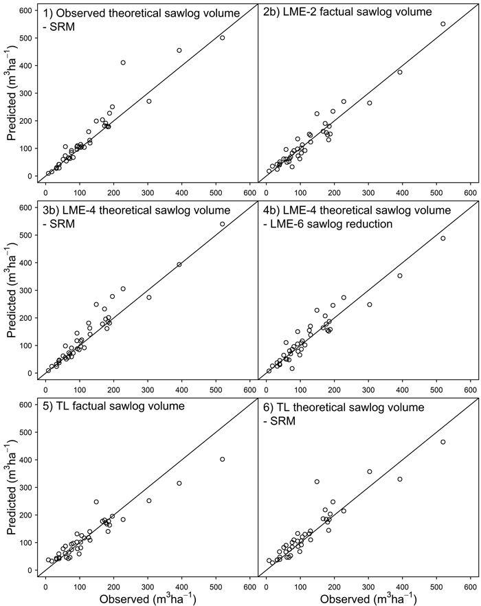
Fig. 1. Observed vs. predicted values for the factual sawlog volume (m3 ha–1) at the stand- level (30 × 30 m). For simplicity, only the b versions of alternatives 2, 3 and 4 are shown. LME = linear mixed-effects model, TL = tree list, SRM = sawlog reduction of Mehtätalo (2002). See Materials and Methods for detailed definitions. The study area is located in boreal forest in eastern Finland and it is dominated by Scots pine.
| Table 7. Root mean squared error (RMSE%) and BIAS% values for the model of Mehtätalo (2002) when estimating the factual sawlog volume with different sets of Scots pines. Subset 1 = pines with factual sawlog volume > 0. Subset 2 = pines with factual sawlog volume > 0, but not flawless. Subset 3 = flawless pines. Subset 4 = all defective pines. The main characteristics of the relative sawlog reduction (%) at the tree-level for both observed and modelled values with different sets of pines are also shown. The study area is located in boreal forest in eastern Finland. |
| RMSE% | BIAS% | MinSR | MaxSR | MeanSR | SdSR |
| Observed | - | - | 0 | 100 | 39.8 | 36.9 |
| All pines (n = 1235) | 73.6 | –18.0 | 15.4 | 63.1 | 32.4 | 10.4 |
| Subset 1 (n = 971) | 38.8 | 1.3 | 15.4 | 58.5 | 31.2 | 10.0 |
| Subset 2 (n = 625) | 43.7 | –15.3 | 15.4 | 58.5 | 30.1 | 9.6 |
| Subset 3 (n = 346) | 30.4 | 27.8 | 16.1 | 58.2 | 33.3 | 10.2 |
| Subset 4 (n = 889) | 96.9 | –46.7 | 15.4 | 63.1 | 32.1 | 10.5 |