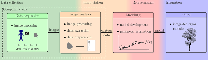
Fig. 1. Overview of the described workflow: showing the steps from photographing leaves to the integration of the resulting organ modules into an existing FSPM.
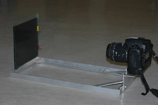
Fig. 2. Recording equipment. The use of an additional black board to cover the shining metal arms is recommended in order to prevent reflections, as well as the use of a second carrying strap fixed near the object plane to prevent toppling and to improve equilibrium for field use.
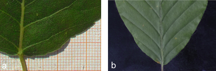
Fig. 3. Edge effects of different backgrounds. a) The photograph clearly shows a wide shadow that would cause problems in case of an automatic segmentation. b) A black velvet as background absorbs nearly all shadows and provides a soft structure allowing the leaf to sink in.
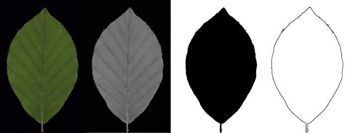
Fig. 4. Schematic workflow of contour extraction: Original image (colour picture) / green channel (grey-value image) / threshold image (black-white picture) / contour picture.
| Table 1. Summary statistics of the three trees that were used to build the data base for this study. From each tree a set of leaves was randomly chosen and observed over the whole period of growth. | ||
| Tree | Number of leaves | Number of measurements |
| T1 | 20 | 262 |
| T2 | 12 | 162 |
| T3 | 11 | 158 |
| Total | 43 | 582 |
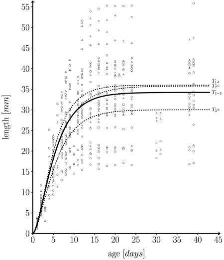
Fig. 5. Fitted length function, based on 582 measurements on a total of 43 individual leaves taken from three different trees (T1 = 262, T2 = 162, T3 = 158 measurements) over one growth period. Solid line: fitted leaf length function over whole data set (T1–3 = T1∪T2∪T3) (Eq. 1; m = 34.224 ± 0.595 (mean ± SD), k = 0.249 ± 0.027, n = 1.859 ± 0.295, l0 = 0); Dashed lines: fitted functions for each individual tree; T1 (triangles), T2 (dots) and T3 (squares): measured leaf data.
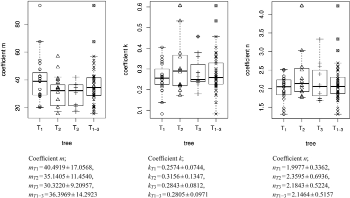
Fig. 6. Overview of the size model coefficients’ m, k and n in box and whisker plots (median, IQR, whiskers at 1.5 IQD or extremal values) broken down to the level of individual leaves (in total 43 leaves) and ordered by tree (T1, T2, T3). The fourth column in each figure illustrates the combined results of all three trees taken together (T1–3 = T1∪T2∪T3), see Table 1. Below we report the mean ± SD of the respective size model coefficients.
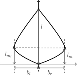
Fig. 7. Depicting the four shape parameters of the proportional model on a leaf contour. See list of symbols for further explanations.
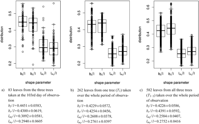
Fig. 8. Distribution of shape parameters in box and whisker plots (median, IQR, whiskers at 1.5 IQD or extremal values) of a) 83 leaves measured on one single day, b) of one tree and c) of all three trees taken together over the whole period of observation. Below we report the mean ± SD of the respective shape parameters. See list of symbols for further explanations.
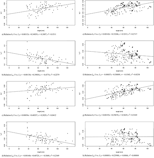
Fig. 9. Linear modelled relation between the model parameters bl / l, br / l, lml / l, lmr / l and the leaf length l of 83 leaves from three trees taken at the 103rd day of observation (sub-figures a–d) and of 262 leaves from one tree taken over the whole period of observation (sub-figures e–h). Correlation coefficient r and multiple R-squared r2. See list of symbols for further explanations. View larger in new window/tab.
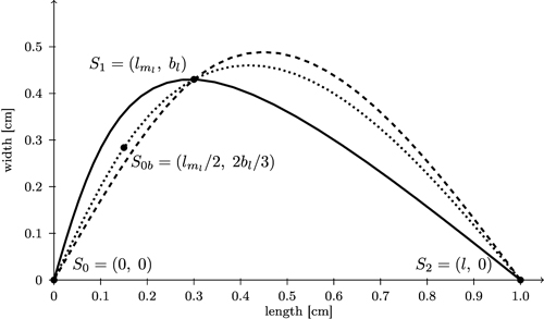
Fig. 10. Comparison of spline interpolation (dashed) between the three support points S0, S1, and S2 which overshoots the maximum width with the bi-interpolation C(s) (solid, black) interpolating splines for contour of the left side of the leaf. Additionally a spline interpolation between four support points (S0b = (lml / 2, 2bl / 3)) is included (dotted).
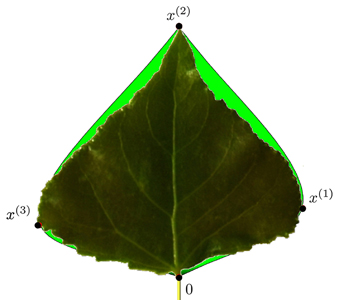
Fig. 11. Modelled contour approximation by bi-interpolation of the proportional model versus the original leaf contour. x(t) are the special contour points used in this model.
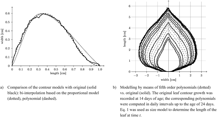
Fig. 12. Reconstruction of a leaf contour over time and comparison of the contour models with original model.
| Table 2. Overview of all models with number of input parameters corresponding to their dimensionality. | ||||||
| Model | Input parameters | |||||
| General | Symmetric | General temporal evolution | ||||
| Proportional | 1+2*2 | = 5 | 1+2 | = 3 | 1+2*4 | = 9 |
| Polynomial | 1+2*6 | = 13 | 1+6 | = 7 | 1+2*6*7 | = 85 |
| Geodesic | 1+2*2 | = 5 | - | 1+4+4 | = 9 | |
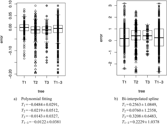
Fig. 13. Error plots [mm2] in box and whisker plots (median, IQR, whiskers at 1.5 IQD or extremal values) of the polynomial and the bi-interpolated spline shape model vs. the original leaf contour of the left leaf side for all individual trees and the average over all trees. The error is calculated as difference between the model and the original leaf contour. The model parameters are individually adapted for each leaf. Below we report the mean ± SD of the respective errors. See list of symbols for further explanations.
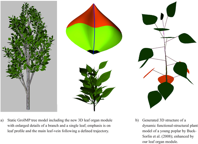
Fig. 14. Two examples integrating the proposed leaf organ module.