Silva Fennica

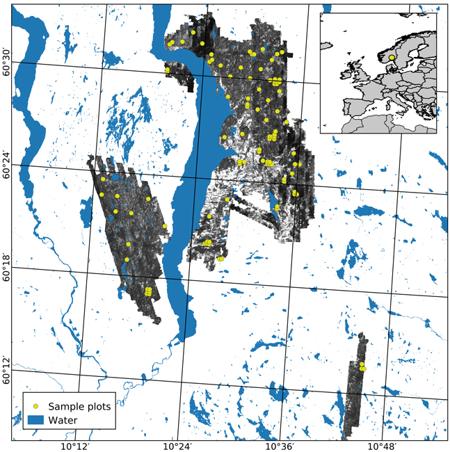
Fig. 1. The geographical location of the study area in Norway (insert) and the extent of the hyperspectral acquisition are shown using an image from the NIR band (708 nm). Sample plots appear in yellow.

Table 1. Summary of volume and species proportions on the 97 sample plots used for training and validation for Spruce (Picea abies), Pine (Pinus sylvestris), Deciduous species (mainly birch (Betula spp.)) and in total. Mean values for all plots are presented in parenthesis.
Species	Species proportion, (mean) (%)	Volume, (mean) in m³ ha^–1
Spruce	1–100 (67)	1–625 (168)
Pine	0–98 (21)	0–369 (48)
Deciduous	0–83 (12)	0–155 (25)
Total		16–625 (241)

Table 2. Summary of number of plots, percent of dominant species of total plot volume and volume for training and validation plots by dominant species; Spruce-dominated (Picea abies), Pine-dominated (Pinus sylvestris), Deciduous-dominated (mainly dominated by Birch (Betula spp.)) and in total. Mean values for all plots are presented in parenthesis.
Dominant species	Number of plots	% of dominant species of total plot volume (mean)	Volume, (mean) in m³ ha^–1
Spruce-dominated	70	45–100 (85)	24–625 (257)
Pine-dominated	22	39–98 (71)	65–471 (227)
Deciduous-dominated	5	53–83 (68)	16–266 (129)
Total	97		16–625 (241)

Table 3. Computation and reference for vegetation indices derived from hyperspectral data and applied in the modelling of species composition.
Index	Computation	Reference
Normalized Difference Vegetation Index		Rouse et al. (1973)
Renormalized Difference Vegetation Index		Roujean and Breon (1995)
Modified red edge Simple Ratio index		Chen (1996)
Conifer Index		Trier et al. (2018)
Spruce Index		Trier et al. (2018)
Soil-Adjusted Vegetation Index		Huete (1988)

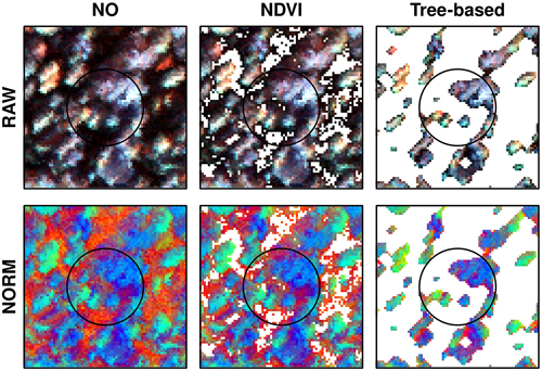
Fig. 2. Example from one field plot applying different normalization (RAW, NORM) and thresholding approaches (NO, NDVI, tree-based). Pixels removed applying thresholding appear white and are not used when computing variables for modelling. Image colors: red = 445 nm, green=714 nm, and blue=839 nm using a linear stretch.

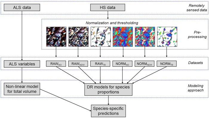
Fig. 3. Schematic diagram of the data processing and modeling steps used in the study. From the remotely sensed data preprocessing is applied to the hyperspectral (HS) data in terms of normalization and thresholding, providing six different datasets for Dirichlet (DR) modelling of species proportions; RAW_NO (no normalization and no thresholding), RAW_NDVI (no normalization and NDVI thresholding), RAW_TB (no normalization and tree-based (TB) thresholding), NORM_NO (normalization and no thresholding), NORM_NDVI (normalization and NDVI thresholding), and NOR_MTB (normalization and TB thresholding). Variables from airborne laser scanning (ALS) data are used in modeling of total volume.

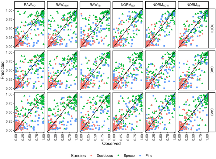
Fig. 4. Observed and predicted species proportions (Spruce = Norway spruce (Picea abies), Pine = Scots pine (Pinus sylvestris), Deciduous (mainly birch (Betula spp.))) for different sensors (CASI, SASI) and their combination (BOTH) for different preprocessing steps (RAW_NO, RAW_NDVI, RAW_TB, NORM_NO, NORM_NDVI, NORM_TB).

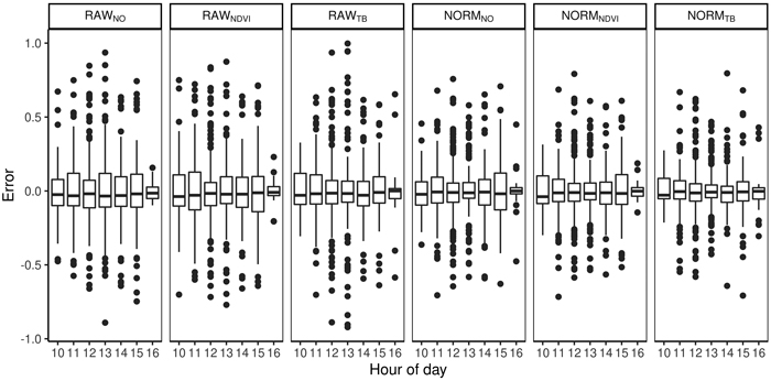
Fig. 5. Difference between predicted and observed species proportions for different hours of the day and for different preprocessing steps (RAW_NO, RAW_NDVI, RAW_TB, NORM_NO, NORM_NDVI, NORM_TB).

Table 4. Results for species-specific volume and fuzzy set accuracy for the Dirichlet regression approach. OA = overall accuracy, RRMSD_S= relative root mean squared error for Norway spruce (Picea abies), RRMSD_P= relative root mean squared error for Scots pine (Pinus sylvestris), RRMSD_D= relative root mean squared error for deciduous trees (mainly birch (Betula spp.)).
Data	Sensor	Kappa-value	OA	RRMSD_S	RRMSD_P	RRMSD_D	Fuzzy set accuracy
Data	Sensor	Kappa-value	OA	RRMSD_S	RRMSD_P	RRMSD_D	Five	Four	Three	Two	One
RAW_NO	CASI	0.53	0.81	48	142.3	142.6	50	73	85	15	11
RAW_NO	SASI	0.39	0.77	42.6	150.6	139.7	45	74	83	18	11
RAW_NO	BOTH	0.53	0.81	46.6	139.5	128	53	76	85	16	10
RAW_NDVI	CASI	0.69	0.87	47.2	148.3	140.8	51	75	86	13	8
RAW_NDVI	SASI	0.43	0.79	41.2	148.6	134.8	47	72	86	14	9
RAW_NDVI	BOTH	0.55	0.82	46.6	146.6	114.7	57	76	86	14	10
RAW_TB	CASI	0.61	0.84	41.2	120.2	107.5	61	83	90	10	6
RAW_TB	SASI	0.57	0.82	48.6	146.3	154.4	48	72	85	15	10
RAW_TB	BOTH	0.52	0.8	48.1	134.7	123.5	57	78	86	14	10
NORM_NO	CASI	0.42	0.77	37.8	135.8	124.6	53	73	85	16	8
NORM_NO	SASI	0.66	0.86	40.6	114.2	148.9	58	78	87	12	6
NORM_NO	BOTH	0.66	0.85	35	117.6	117.6	64	81	90	9	5
NORM_NDVI	CASI	0.62	0.85	35.4	131.5	129.4	60	76	87	13	5
NORM_NDVI	SASI	0.65	0.86	37.7	120.6	124	58	81	91	8	5
NORM_NDVI	BOTH	0.79	0.91	32.4	104.9	109.6	68	84	93	6	2
NORM_TB	CASI	0.76	0.9	36.6	105	100	66	85	92	8	4
NORM_TB	SASI	0.69	0.87	38.1	122.9	132.3	64	82	92	8	6
NORM_TB	BOTH	0.70	0.88	34.2	87	102.2	68	88	93	6	2

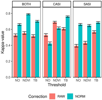
Fig. 6. Kappa values and confidence intervals for dominant species obtained by different sensors (CASI and SASI) and their combination (BOTH). In addition, the different preprocessing steps, i.e., using raw data (RAW) or normalized data (NORM) and different thresholding methods (NO, NDVI or TB).

Table 5. Error matrices of the dominant species classification (S = Norway spruce (Picea abies), P = Scots pine (Pinus sylvestris), D = deciduous (mainly birch (Betula spp.))) obtained from the Dirichlet regression for different sensors (CASI, SASI and combined BOTH) and preprocessing methods (Data). PA = producer’s accuracy and UA = User’s accuracy.
Data	Sensor	CASI				SASI				BOTH
Data	Species	S	P	D	PA	S	P	D	PA	S	P	D	PA
RAW_NO	S	65	11	1	84.4	66	13	2	81.5	65	10	2	84.4
	P	3	10	0	76.9	2	6	0	75.0	3	11	0	78.6
	D	2	1	4	57.1	2	3	3	37.5	2	1	3	50.0
	UA	92.9	45.5	80.0	81.4	94.3	27.3	60.0	77.3	92.9	50.0	60.0	81.4
RAW_NDVI	S	64	6	0	91.4	67	15	1	80.7	65	12	0	84.4
	P	4	15	0	78.9	1	6	0	85.7	3	10	0	76.9
	D	2	1	5	62.5	2	1	4	57.1	2	0	5	71.4
	UA	91.4	68.2	100.0	86.6	95.7	27.3	80.0	79.4	92.9	45.5	100.0	82.5
RAW_TB	S	63	6	2	88.7	65	9	1	86.7	63	8	3	85.1
	P	6	15	0	71.4	3	11	0	78.6	5	13	0	72.2
	D	1	1	3	60.0	2	2	4	50.0	2	1	2	40.0
	UA	90.0	68.2	60.0	83.5	92.9	50.0	80.0	82.5	90.0	59.1	40.0	80.4
NORM_NO	S	63	13	1	81.8	64	5	2	90.1	61	4	1	92.4
	P	5	8	0	61.5	2	16	0	88.9	4	17	0	81.0
	D	2	1	4	57.1	4	1	3	37.5	5	1	4	40.0
	UA	90.0	36.4	80.0	77.3	91.4	72.7	60.0	85.6	87.1	77.3	80.0	84.5
NORM_NDVI	S	65	9	1	86.7	65	5	3	89.0	66	3	0	95.7
	P	3	13	0	81.2	3	16	0	84.2	1	17	0	94.4
	D	2	0	4	66.7	2	1	2	40.0	3	2	5	50.0
	UA	92.9	59.1	80.0	84.5	92.9	72.7	40.0	85.6	94.3	77.3	100.0	90.7
NORM_TB	S	66	3	1	94.3	65	4	2	91.5	66	5	2	90.4
	P	3	17	0	85.0	2	16	0	88.9	1	16	0	94.1
	D	1	2	4	57.1	3	2	3	37.5	3	1	3	42.9
	UA	94.3	77.3	80.0	89.7	92.9	72.7	60.0	86.6	94.3	72.7	60.0	87.6

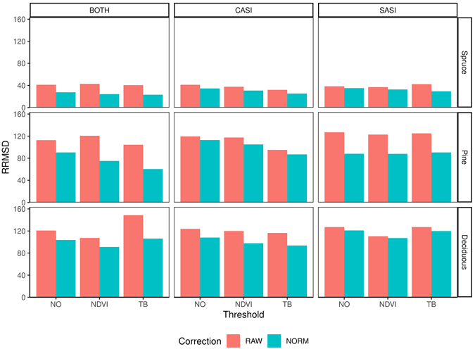
Fig. 7. Relative root mean square difference (RRMSD) for different preprocessing steps, i.e., using raw data (RAW) or normalized data (NORM), and thresholding methods (NO, NDVI, TB), species (Spruce = Norway spruce (Picea abies), Pine = Scots pine (Pinus sylvestris), Deciduous (mainly birch (Betula spp.))), sensors (CASI and SASI) and their combination (BOTH).

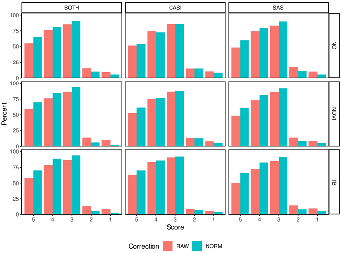
Fig. 8. Percentage of observations in different score values (5–1) obtained from fuzzy validation by different sensors (CASI and SASI) and their combination (BOTH). In addition, the different preprocessing steps, i.e., using raw data (RAW) or normalized data (NORM) and different thresholding methods (NO, NDVI or TB). A score of 5 indicates no deviation between predicted and observed species proportion and a lower score indicates subsequent higher deviation; for details see section 2.4.3.

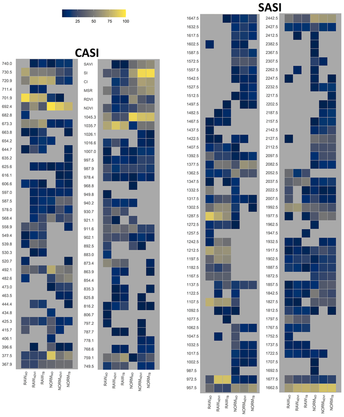
Fig. 9. Relative importance of HS-derived variables, i.e., vegetation index name or wavelength obtained by different sensors (CASI and SASI) and the different preprocessing steps, i.e., using raw data (RAW) or normalized data (NORM) and different thresholding methods (NO, NDVI or TB). Importance was computed as the percentage the variable was selected in the cross-validation. View larger in new window/tab.