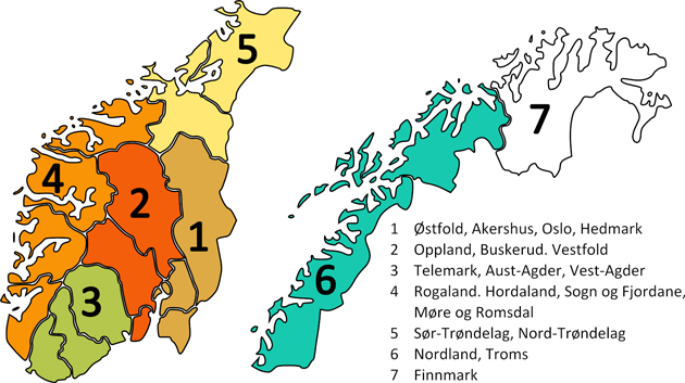
Fig. 1. Norwegian forest inventory (NFI) regions. The analyses cover region 1 through 6. Region 7 is excluded from the analyses due to lack of data. The names of the counties comprising each region in the study period are shown to the right.
| Table 1. Descriptive statistics of forest and forestry conditions in the six regions covered by the analyses. Data is from the middle of the study period (1996–2016). Source: Statistics Norway (2018b); Statistics Norway (2018d); Statistics Norway (2018e); Statistics Norway (2018f); Statistics Norway (2018g). | |||||||
| Region/Counties1 | Forest area, km2 | Growing stock, Mm3 | Share mature forest | Annual harvest, 1000 m3 | Average property size, ha | Harvest intensity, m3 ha–1 | |
| All | 79 955 | 746 | 38% | 7801 | 68 | 1.0 | |
| 1 | Østfold, Akershus, Oslo, Hedmark | 19 718 | 211 | 30% | 3384 | 93 | 1.7 |
| 2 | Oppland, Buskerud, Vestfold | 15 430 | 158 | 36% | 2280 | 72 | 1.5 |
| 3 | Telemark, Aust-Agder, Vest-Agder | 11 923 | 131 | 43% | 1024 | 74 | 0.9 |
| 4 | Rogaland, Hordaland, Sogn og Fjordane, Møre og Romsdal | 10 552 | 106 | 40% | 268 | 39 | 0.3 |
| 5 | Sør-Trøndelag, Nord-Trøndelag | 10 901 | 86 | 40% | 717 | 81 | 0.7 |
| 6 | Nordland, Troms | 11 432 | 54 | 47% | 128 | 63 | 0.1 |
| 1 As of January 1, 2020 some of the counties were merged in a regional reform. Some of the counties in regions 1–3 were merged across regions. The regions are so far not adjusted in the NFI data as reported by Statistics Norway. | |||||||
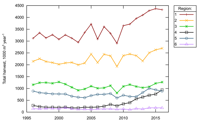
Fig. 2. Total industrial harvest in the six regions for which the analyses cover, 1000 m3 year–1. Source: Statistics Norway (2018b).
| Table 2. Correlation (Pearson correlation coefficient) between variables used in the timber supply analyses. Variables are not transformed (i.e. not in log-form). | ||||||
| Sawlog harvest | Pulpwood harvest | Sawlog price | Pulpwood price | Standing stock | Interest rate | |
| Sawlog harvest | 1.00 | 0.97 | 0.36 | –0.07 | 0.93 | –0.08 |
| Pulpwood harvest | 0.97 | 1.00 | 0.36 | –0.03 | 0.92 | –0.08 |
| Sawlog price | 0.36 | 0.36 | 1.00 | 0.73 | 0.16 | 0.50 |
| Pulpwood price | –0.07 | –0.03 | 0.73 | 1.00 | –0.25 | 0.72 |
| Standing stock | 0.93 | 0.92 | 0.16 | –0.25 | 1.00 | –0.20 |
| Interest rate | –0.08 | –0.08 | 0.50 | 0.72 | –0.20 | 1.00 |
| Table 3. Poolability F-tests (F-value and significance level) of timber supply models with regional own price elasticities. The null hypothesis is that all regional price elasticities are equal within each model. | |||
| Fixed effect | Random effect | First difference | |
| Pulpwood | |||
| Static | 7.2*** | 7.4*** | 0.9 |
| Dynamic | 2.9** | 4.7*** | 1.3 |
| Sawlogs | |||
| Static | 21.8*** | 21.9*** | 0.6 |
| Dynamic | 5.3*** | 4.9*** | 0.8 |
| Significance levels: *** = 1%, ** = 5%, * = 10% | |||
| Table 4. Parameter estimates, standard errors (in parenthesis), and significance level indicators for pulpwood supply models. | |||
| Model | Fixed effect | Random effect | First difference |
| Static, common slope | |||
| Intercept | –6.20 (5.11) | ||
| Pulpwood price | 0.53 (0.37) | 0.58 (0.34)* | 0.50 (0.19)*** |
| Sawlog price | 0.04 (0.23) | 0.15 (0.25) | 0.04 (0.13) |
| Standing stock | 1.05 (0.53)** | 1.28 (0.38)*** | 0.85 (0.27)*** |
| Rate of return | –2.05 (1.07)* | –1.71 (1.36) | –0.39 (0.94) |
| Dynamic, common slope | |||
| Intercept | –4.38 (1.10)*** | ||
| Pulpwood price | 0.24 (0.14) | 0.15 (0.15) | 0.53(0.21)** |
| Sawlog price | 0.27 (0.10)*** | 0.11 (0.08) | 0.17(0.16) |
| Standing stock | 0.86 (0.20)*** | 0.45 (0.04)*** | –0.03(0.72) |
| Rate of return | –0.53 (0.79) | –1.28 (0.85) | –0.88(1.32) |
| Pulpwood harvest, t–1 | 0.81 (0.04)*** | 0.82 (0.03)*** | –0.08(0.07) |
| Static, regional slopes | |||
| Intercept | 1.57 (6.28) | ||
| Pulpwood price, region 1 | 0.04 (0.38) | 0.14 (0.36) | 0.30 (0.07)*** |
| Pulpwood price, region 2 | 0.53 (0.35) | 0.53 (0.34) | 0.57 (0.07)*** |
| Pulpwood price, region 3 | 1.59 (0.44)*** | 1.45 (0.42)*** | 1.00 (0.06)*** |
| Pulpwood price, region 4 | –0.35 (0.57) | –0.26 (0.54) | 0.52 (0.12)*** |
| Pulpwood price, region 5 | 0.35 (0.39) | 0.37 (0.38) | 0.23 (0.10)** |
| Pulpwood price, region 6 | 0.96 (0.56)* | 0.85 (0.53) | 0.13 (0.12) |
| Sawlog price | –0.22 (0.33) | –0.18 (0.31) | 0.02 (0.13) |
| Standing stock | 0.79 (0.46)* | 0.83 (0.46)* | 0.82 (0.31)*** |
| Rate of return | –2.34 (1.13)** | –2.27 (1.14)** | –0.19 (0.99) |
| Dynamic, regional slopes | |||
| Intercept | –8.45 (3.41)** | ||
| Pulpwood price, region 1 | 0.20 (0.12) | 0.21 (0.11)* | 0.44(0.13)*** |
| Pulpwood price, region 2 | 0.26 (0.08)*** | 0.26 (0.08)*** | 0.59(0.1)*** |
| Pulpwood price, region 3 | 0.77 (0.09)*** | 0.67 (0.09)*** | 1.05(0.15)*** |
| Pulpwood price, region 4 | –0.16 (0.23) | –0.08 (0.20) | 0.52(0.14)*** |
| Pulpwood price, region 5 | 0.04 (0.11) | 0.08 (0.11) | 0.24(0.26) |
| Pulpwood price, region 6 | 0.39 (0.13)*** | 0.36 (0.13)*** | 0.11(0.31) |
| Sawlog price | 0.17 (0.10)* | 0.19 (0.09)** | 0.13(0.17) |
| Standing stock | 0.81 (0.19)*** | 0.82 (0.20)*** | –0.53(0.83) |
| Rate of return | –0.74 (0.70) | –0.71 (0.71) | –0.65(1.38) |
| Pulpwood harvest, t–1 | 0.70 (0.07)*** | 0.72 (0.06)*** | –0.08(0.1) |
| Significance levels: *** = 1%, ** = 5%, * = 10% | |||
| Table 5. Parameter estimates, standard errors (in parenthesis), and significance level indicators for sawlog supply models. | |||
| Model | Fixed effect | Random effect | First difference |
| Static, common slope | |||
| Intercept | –11.14 (4.20)*** | ||
| Pulpwood price | –0.32 (0.27) | –0.27 (0.23) | 0.02 (0.14) |
| Sawlog price | 0.76 (0.23)*** | 0.88 (0.30)*** | 1.24 (0.13)*** |
| Standing stock | 1.50 (0.58)** | 1.73 (0.41)*** | 2.09 (0.32)*** |
| Rate of return | 1.60 (0.77)** | 1.95 (0.99)* | –1.44 (0.78)* |
| Dynamic, common slope | |||
| Intercept | –4.22 (2.03)** | ||
| Pulpwood price | –0.30 (0.15)* | –0.36 (0.09)*** | 0.23(0.15) |
| Sawlog price | 0.76 (0.13)*** | 0.64 (0.26)** | 1.01(0.08)*** |
| Standing stock | 0.75 (0.12)*** | 0.41 (0.17)** | 2.22(0.65)*** |
| Rate of return | 0.47 (0.63) | –0.17 (0.68) | –0.58(0.81) |
| Sawlog harvest, t–1 | 0.78 (0.16)*** | 0.82 (0.08)*** | –0.31(0.09)*** |
| Static, regional slopes | |||
| Intercept | 5.83 (1.65)*** | ||
| Pulpwood price | –0.57 (0.17)*** | –0.56 (0.18)*** | 0.04 (0.13) |
| Sawlog price, region 1 | 0.79 (0.09)*** | 0.79 (0.09)*** | 1.04 (0.03)*** |
| Sawlog price, region 2 | 0.72 (0.10)*** | 0.72 (0.11)*** | 1.30 (0.05)*** |
| Sawlog price, region 3 | 0.98 (0.12)*** | 0.97 (0.11)*** | 1.21 (0.04)*** |
| Sawlog price, region 4 | –2.67 (0.21)*** | –2.49 (0.19)*** | 0.74 (0.08)*** |
| Sawlog price, region 5 | 1.62 (0.12)*** | 1.57 (0.12)*** | 1.20 (0.04)*** |
| Sawlog price, region 6 | 0.53 (0.12)*** | 0.54 (0.12)*** | 1.77 (0.04)*** |
| Standing stock | 0.64 (0.24)*** | 0.69 (0.26)*** | 2.09 (0.31)*** |
| Rate of return | 1.03 (0.81) | 1.06 (0.81) | –1.45 (0.79)* |
| Dynamic, regional slopes | |||
| Intercept | –3.02 (3.67) | ||
| Pulpwood price | –0.47 (0.18)*** | –0.42 (0.18)** | 0.19(0.16) |
| Sawlog price, region 1 | 0.78 (0.07)*** | 0.76 (0.08)*** | 0.88(0.09)*** |
| Sawlog price, region 2 | 0.80 (0.07)*** | 0.78 (0.08)*** | 1.07(0.12)*** |
| Sawlog price, region 3 | 0.95 (0.09)*** | 0.91 (0.10)*** | 0.76(0.25)*** |
| Sawlog price, region 4 | –1.26 (0.68)* | –0.75 (0.56) | 0.81(0.14)*** |
| Sawlog price, region 5 | 1.19 (0.20)*** | 1.06 (0.20)*** | 0.94(0.21)*** |
| Sawlog price, region 6 | 0.76 (0.10)*** | 0.77 (0.08)*** | 1.72(0.15)*** |
| Standing stock | 0.59 (0.16)*** | 0.63 (0.15)*** | 2.11(0.63)*** |
| Rate of return | 0.73 (0.64) | 0.66 (0.63) | –0.85(0.77) |
| Sawlog harvest, t–1 | 0.50 (0.18)*** | 0.57 (0.19)*** | –0.30(0.1)*** |
| Significance levels: *** = 1%, ** = 5%, * = 10% | |||
| Table 6. Unconstrained OLS and seemingly unrelated regression (SUR) pulpwood and sawlog supply models. Parameter estimates, standard errors (in parenthesis), and significance level indicators for first difference models. | ||||
| Elasticity | Pulpwood | Sawlog | ||
| Unconstrained OLS | Constrained SUR | Unconstrained OLS | Constrained SUR | |
| Own price, region 1 | 0.35 (0.34) | 0.30 (0.30) | 1.02 (0.36)*** | 0.90 (0.33)*** |
| Own price, region 2 | 0.61 (0.35)* | 0.50 (0.31) | 1.32 (0.38)*** | 1.21 (0.35)*** |
| Own price, region 3 | 1.00 (0.33)*** | 0.96 (0.30)*** | 1.21 (0.38)*** | 1.30 (0.34)*** |
| Own price, region 4 | 0.58 (0.37) | 0.79 (0.33)** | 0.80 (0.55) | 0.88 (0.50)* |
| Own price, region 5 | 0.16 (0.38) | 0.34 (0.33) | 1.12 (0.42)** | 0.97 (0.39)** |
| Own price, region 6 | 0.02 (0.40) | 0.46 (0.37) | 1.83 (0.42)*** | 1.85 (0.38)*** |
| Cross price | 0.01 (0.17) | 0.05 (0.17) | 0.03 (0.18) | –0.06 (0.17) |
| Standing stock, region 1 | 1.77 (1.90) | 1.39 (1.65) | 1.25 (1.97) | 1.39 (1.65) |
| Standing stock, region 2 | 1.73 (2.37) | 1.84 (2.05) | 2.66 (2.40) | 1.84 (2.05) |
| Standing stock, region 3 | 0.83 (1.52) | 1.29 (1.32) | 1.98 (0.59) | 1.29 (1.32) |
| Standing stock, region 4 | 1.24 (1.05) | 1.86 (0.91)** | 2.40 (1.09)** | 1.86 (0.91)** |
| Standing stock, region 5 | 0.02 (1.19) | 0.36 (1.44) | 0.66 (1.71) | 0.36 (1.44) |
| Standing stock, region 6 | –0.19 (0.95) | 1.42 (1.19) | 2.86 (1.43)** | 1.42 (1.19) |
| Rate of return | –0.16 (1.01) | –0.83 (0.84) | –1.46 (1.04) | –0.83 (0.84) |
| Significance levels: *** = 1%, ** = 5%, * = 10% | ||||