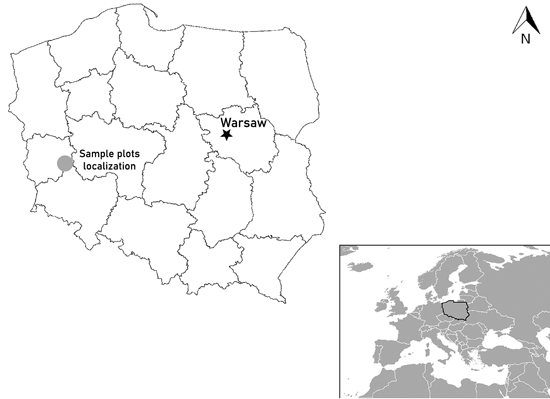
Fig. 1. Location of black locust sample plots in west Poland.
| Table 1. Summary characteristics of the black locust sample plots located in west Poland: average stand age (A, years), sample plot area (P, m2), stocking (N, trees ha–1), basal area at breast height (BA, m2 ha–1), average diameter at breast height (Dg, cm), and average height (Hg, m). | |||||
| Minimum | Maximum | Mean | Median | Stand. Dev. | |
| A | 16 | 85 | 50 | 50 | 21 |
| P | 864 | 5944 | 2359 | 1914 | 1278 |
| N | 167 | 1134 | 586 | 507 | 304 |
| BA | 10.06 | 40.52 | 21.73 | 20.53 | 7.72 |
| Dg | 11.47 | 43.94 | 23.94 | 25.23 | 9.08 |
| Hg | 9.84 | 27.19 | 20.3 | 21.18 | 5.19 |
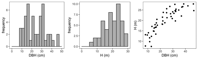
Fig. 2. Diameter at breast height (DBH) distribution (left), height distribution (H, middle) and H-DBH relationship (right) of black locust sample trees.
| Table 2. Characteristics of black locust sample trees. Diameter at breast height (DBH, cm), tree height (H, m), section diameter over bark (D, cm), section diameter under bark (d, cm) and reference tree volume over bark (VR, m3). | |||||
| Minimum | Maximum | Mean | Median | Stand. Dev. | |
| DBH | 8.1 | 46.7 | 24.05 | 22.98 | 10.29 |
| H | 7.5 | 27.9 | 19.99 | 20.7 | 5.54 |
| D | 0.3 | 54.8 | 16.19 | 15.35 | 10.13 |
| d | 0.15 | 49.25 | 13.93 | 13.30 | 8.57 |
| VR | 0.0212 | 1.8056 | 0.5421 | 0.3959 | 0.4681 |
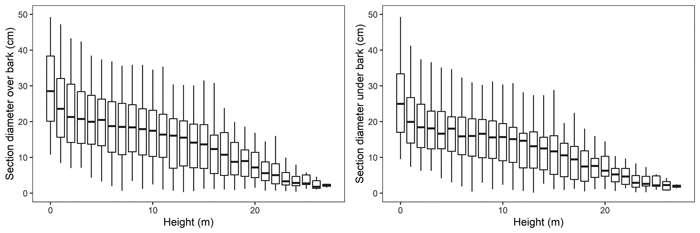
Fig. 3. Black locust sample trees section diameters over bark (left) and under bark (right).
| Table 3. Goodness-of-fit measures for the analysed fixed-effects taper models for black locust: R2 – coefficient of determination (Eq. 8), ME – mean error (Eq. 9), and AIC – Akaike information criterion (Eq. 10). Model nr. 1 – Newberry and Burkhart 1986, nr. 2 – Biging 1984, nr. 3 – Riemer et al. 1995, nr. 4 – Demaerschalk 1972, nr. 5 – Lee et al. 2003, nr. 6 – Muhairwe 1999 and nr. 7 – Kozak 1997. | |||||||
| section diameter over bark | |||||||
| Model nr. | 1 | 2 | 3 | 4 | 5 | 6 | 7 |
| R2 | 0.929 | 0.926 | 0.718 | 0.933 | 0.959 | 0.958 | 0.962 |
| ME | 12.212 | 12.533 | 20.327 | 1.547 | 3.176 | 1.535 | –1.528 |
| AIC | 11916 | 11955 | 13261 | 11859 | 11392 | 11404 | 11312 |
| section diameter under bark | |||||||
| R2 | 0.925 | 0.923 | 0.777 | 0.928 | 0.959 | 0.96 | 0.965 |
| ME | 8.461 | 8.864 | 11.682 | 1.552 | 4.33 | 3.229 | –1.05 |
| AIC | 9225 | 9250 | 10093 | 9197 | 8754 | 8737 | 8643 |
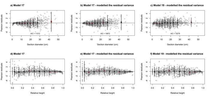
Fig. 4. Residuals plots for elaborated black locust fixed-effect taper model (Eq. 17, a, b, d, e) and mixed-effect taper model (Eq. 19, c, f) achieved for section diameter over bark according to the section diameter (upper part) and relative height (lower part). Grey dots define the Pearson residuals and large black dots show the means of the residuals in 10 classes of section diameter (upper part) and relative height (lower part). Thin vertical lines show the confidence interval of individual observations (mean ± 1.96 SD), and thick vertical lines (inside black dots) show the 95% confidence interval of the class mean. View larger in new window/tab.
| Table 4. The parameter estimates and standard errors (in brackets) of the fixed-effects taper model (Eq. 17 and 18) and mixed-effects taper model (Eq. 19) for black locust. | |||||
| Parameter | Fixed-effects taper model | Mixed-effects taper model | |||
| section diameter over bark | section diameter under bark | section diameter over bark | section diameter under bark | ||
| b1 | 0.962 (0.026) | 0.629 (0.057) | –1.046 (0.105) | –0.917 (0.137) | |
| b2 | 0.983 (0.008) | 1.048 (0.023) | 0.926 (0.033) | 0.881 (0.072) | |
| b3 | - | - | 0.041 (0.031) | 0.081 (0.054) | |
| b4 | 0.289 (0.013) | 0.26 (0.015) | 0.262 (0.011) | 0.256 (0.009) | |
| b5 | –7.643 (0.763) | –7.565 (0.772) | 9.669 (1.031) | 9.483 (0.585) | |
| b6 | - | - | 2.944 (0.641) | 3.858 (0.547) | |
| b7 | - | 2.949 (0.67) | –2.041 (0.541) | –3.379 (0.814) | |
| b8 | 0.061 (0.005) | 0.047 (0.005) | –0.134 (0.017) | –0.142 (0.014) | |
| Plot level | sd(β1) | - | - | 0.009 | - |
| sd(β2) | - | - | 2.932 | - | |
| sd(β3) | - | - | 0.032 | - | |
| corr (β1, β2) | - | - | 0.520 | - | |
| corr (β1, β3) | - | - | 0.517 | - | |
| corr (β2, β3) | - | - | 1 | - | |
| Tree level | sd(β1) | - | - | 0.012 | 0.023 |
| sd(β2) | - | - | 0.722 | 1.911 | |
| sd(β3) | - | - | 0.056 | 0.061 | |
| corr (β1, β2) | - | - | 1 | 0.779 | |
| corr (β1, β3) | - | - | 1 | 0.781 | |
| corr (β2, β3) | - | - | 1 | 1 | |
| σ2 | - | - | 0.1152 | 0.0812 | |
| 1.345 | 1.331 | 1.843 | 1.823 | ||
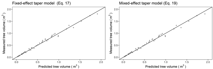
Fig. 5. Relationship between the reference (true) tree volume and predicted tree volume using the fixed-effects taper model (Eq. 17, left) and mixed-effects taper model (Eq. 19, right) for black locust.
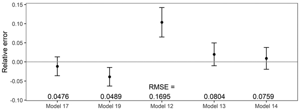
Fig. 6. 95% confidence intervals for the relative errors achieved during volume prediction based on all analysed volume equations for black locust. Model 17 – fixed-effects taper model (Eq. 17), Model 19 – mixed-effects taper model (Eq. 19), Model 12 – Moshki and Lamersdorf 2011 (Eq. 12), Model 13 – Sopp and Kolozs 2000 (Eq. 13), Model 14 – Lockow and Lockow 2015 (Eq. 14).