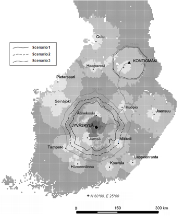
Fig. 1. Study area around the city of Jyväskylä (Scenarios 1 & 2) and around the satellite terminal of Kontiomäki (Scenario 3).
| Table 1. Main and sub-scenarios used in the study. Past (max. 60 tonnes) and current (max. 64 tonnes) road transport dimensions for traditional and container supply chains were compared. Additional sub-scenarios for current dimensions treat alternative numbers of trucks and wagons. Main scenarios: Sce. 1 = current use, Sce. 2 = additional use (by truck), and Sce. 3 = additional use (by train). | |||
| Sub-scenarios | Main scenarios | ||
| Sce. 1 | Sce. 2 | Sce. 3 | |
| Traditional | |||
| Past dimensions | 1.1.1 | 2.1.1 | 3.1.1 |
| Current dimensions | 1.1.2 | 2.1.2 | 3.1.2 |
| a. Sub-scenario | 1.1.3 | 2.1.2 | 3.1.3 |
| b. Sub-scenario | 3.1.4 | ||
| Container | |||
| Past dimensions | 1.2.1 | 2.2.1 | 3.2.1 |
| Current dimensions | 1.2.2 | 2.2.2 | 3.2.2 |
| a. Sub-scenario | 1.2.3 | 2.2.3 | 3.2.3 |
| b. Sub-scenario | 3.2.4 | ||
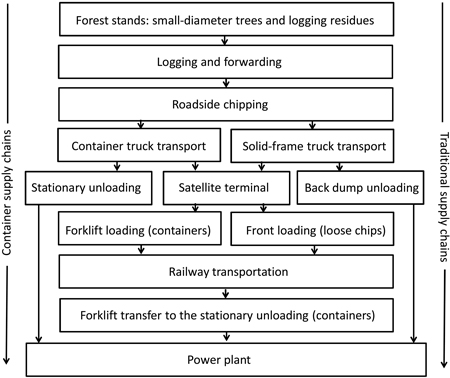
Fig. 2. Process description of material flows and handling operations of the supply chains studied.
| Table 2. Target demand of case power plant for forest chips (GWh). Sce. 1 = current use, Sce. 2 = additional use (by truck), and Sce. 3 = additional use (by train). | |||
| Biomass demand, GWh | |||
| Sce. 1 | Sce. 2 | Sce. 3 | |
| Base demand of Sce. 1 | - | 540 | 540 |
| Logging residues | 300 | 80 | 100 |
| Small-diameter trees | 240 | 120 | 100 |
| Total | 540 | 740 | 740 |
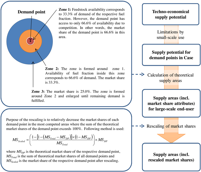
Fig. 3. Description of availability analysis for forest biomass in a competitive market (Korpinen et al. 2012).
| Table 3. Used purchase price and annual costs of machines and vehicles used in the simulation model. Prices and costs are presented without Value Added Tax (VAT, 0%). | |||
| Cost element | Purchased price, € | Annual fixed cost, €/a | Variable cost, €/unit |
| Truck transport (Sce. 1, 2 and 3) | |||
| Roadside chipper | 450 000 | 285 000 | 3 €/tn |
| Container truck | 270 000 | 83 000 | 0.012 €/tnkm |
| Unloading machine | 85 000 | 57 519 | 11.07 €/container |
| Solid-frame truck | 265 000 | 86 000 | 0.012 €/tnkm |
| Railway transport (Sce. 3) | |||
| Locomotive and wagons | 2 200 000 | 319 039 | |
| Intermodal composite container | 15 000 | 5400 | 0.016 €/tnkm |
| Metal container | 8390 | 3036 | 0.013 €/tnkm |
| Front-loader | 205 000 | 154 202 | - |
| Forklift loader | 250 000 | 179 023 | - |
| Unloading machine | 85 000 | 57 519 | 11.07 €/container |
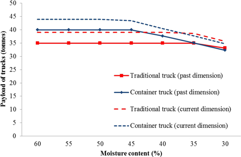
Fig. 4. Payload of forest chips (tonnes) for traditional trucks and container trucks based on past and current dimensions and the moisture content of forest chips.
| Table 4. Railway transportation cost structure components (%-share) as an example for intermodal composite and interchangeable metal containers. | |||
| %-share | Cost component | Metal containers | Intermodal composite containers |
| Fixed costs | Locomotive and wagons | 15 | 11 |
| Rail infra | 13 | 9 | |
| Containers | 16 | 36 | |
| Variable cost | Operational cost (363 km) | 40 | 33 |
| Gross tonne cost | 10 | 7 | |
| Maintenance | 5 | 4 | |
| Total cost | 100 a) | 100 a) | |
| a) Total annual cost of railway transportation (180 trips and 20 wagons) was 1 136 000 € for metal containers and 1 586 000 € for intermodal composite containers. | |||
| Table 5. Average efficiency (minutes/unit) of loading and unloading (Sce. 1, 2 and 3). | ||
| Transport option | Efficiency, minutes/unit | |
| Loading (min–max) | Unloading (min–max) | |
| Truck transport | ||
| Traditional truck | ||
| Sce. 1 and 2 | 50–80/truck | 25–35/truck |
| Sce. 3 (terminals) | 50–80/truck | 25–35/truck |
| Container truck | ||
| Sce. 1 and 2 | 50–80/truck | 8–10/container |
| Sce. 3 (terminals) | 50–80/truck | 4–6/container |
| Railway transport | ||
| Intermodal composite container | 1–3/container | 5–7/container |
| Metal container | 2–3/container | 5–7/container |
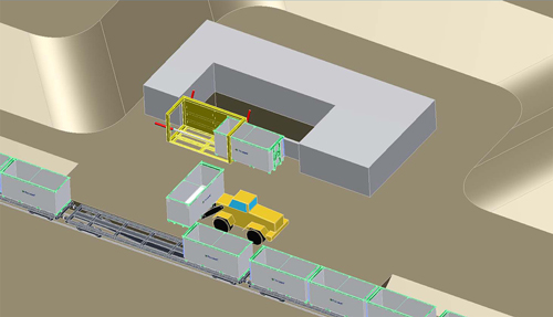
Fig. 5. Stationary unloading machine with forklift loader to transfer composite containers from a train (Fibrocom Ltd., Supercont®).
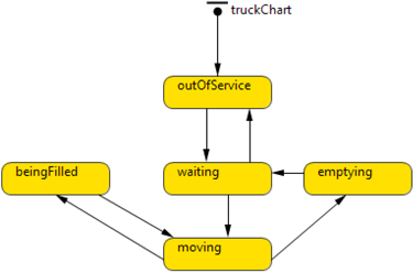
Fig. 6. State chart for the truck agents.
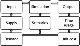
Fig. 7. Simulation process description consisting of input (supply and demand) and output (time usage and unit cost) data for chosen scenarios.
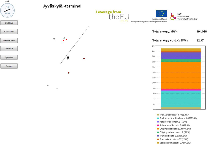
Fig. 8. Screen shot from the display of the simulation model used in the study.
| Table 6. Roadside cost of logging residues and small-sized trees used in this study (€/MWh). | |||||
| Cost (€/MWh) | Overhead cost | Stumpage price | Logging cost | Forwarding cost | Total roadside cost |
| Logging residues | 0.5 | 0.5 | 0.2 | 2.9 | 4.1 |
| Small-diameter trees | 1.0 | 3.0 | 9.1 | 2.7 | 15.8 |
| Table 7. Number of trucks used to fulfil the demand target of the scenarios in the simulation model. | ||||
| Number of trucks and wagons in the demand target of the scenarios | Sce. 1 (trucks) | Sce. 2 (trucks) | Sce. 3 (trucks) | (wagons) |
| Traditional truck | ||||
| Past dimensions | 10 | 18 | 14 | 20 |
| Current dimensions | 8 | 14 | 12 | 20 |
| a. Sub-scenario | 10 | 16 | 12 | 15 |
| b. Sub-scenario | 14 | 15 | ||
| Container truck | ||||
| Past dimensions | 8 | 12 | 12 | 20 |
| Current dimensions | 6 | 10 | 10 | 20 |
| a. Sub-scenario | 8 | 12 | 12 | 20 |
| b. Sub-scenario | 12 | 15 | ||
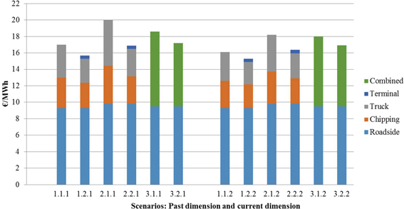
Fig. 9. Unit cost of forest chips (€/MWh) transported by traditional supply chain and container supply chain (past and current dimension). Combined system includes both truck and railway supply chains. Scenarios are presented in Table 1.
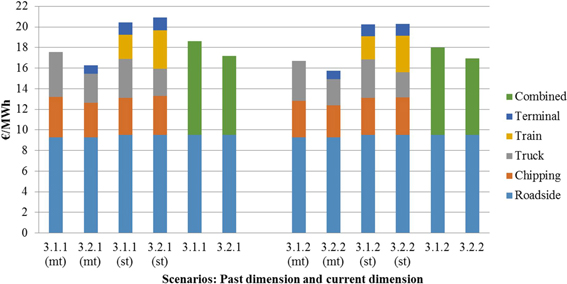
Fig. 10. Unit cost of forest chips (€/MWh) transported by traditional supply chain and container supply chain as calculated separately for the truck and railway supply chain (past and current dimension). Main terminal (around power plant) = mt; satellite terminal (around railway terminal) = st. Scenarios are presented in Table 1.
| Table 8. Simulated delivery and cost results of traditional and container supply chains for forest chips based on current dimension scenarios. Target demand results (200, 540 and 740 GWh/a) are also included. Scenarios are presented in Table 1. | |||||
| Scenarios | Delivery | Cost | |||
| Main scenarios | Sub-scenarios | Total, GWh/a | Railway, GWh/a | milj. €/a | €/MWh |
| Traditional | |||||
| Sce. 1 | 540 | 8.7 | 16.2 | ||
| 1.1.2 | 537 | 8.6 | 16.1 | ||
| 1.1.3 | 637 | 10.4 | 16.4 | ||
| Sce. 2 | 740 | 13.6 | 18.3 | ||
| 2.1.2 | 730 | 13.3 | 18.2 | ||
| 2.1.3 | 787 | 14.7 | 18.6 | ||
| Sce. 3 | 740 | 13.8 | 18.7 | ||
| 200 | (4.7) | (23.3) | |||
| 3.1.2 | 721 | 13.0 | 18.0 | ||
| 237 | (4.8) | (20.2) | |||
| 3.1.3 | 661 | 13.2 | 20.0 | ||
| 178 | (4.7) | (26.5) | |||
| 3.1.4 | 757 | 13.8 | 18.2 | ||
| 178 | (4.4) | (24.8) | |||
| Container | |||||
| Sce. 1 | 540 | 8.3 | 15.4 | ||
| 1.2.2 | 482 | 7.4 | 15.3 | ||
| 1.2.3 | 638 | 9.7 | 15.3 | ||
| Sce. 2 | 740 | 11.9 | 16.1 | ||
| 2.2.2 | 709 | 11.6 | 16.3 | ||
| 2.2.3 | 834 | 13.7 | 16.4 | ||
| Sce. 3 | 740 | 12.4 | 16.7 | ||
| 200 | (4.4) | (22.2) | |||
| 3.2.2 | 654 | 11.1 | 16.9 | ||
| 226 | (4.6) | (20.3) | |||
| 3.2.3 | 788 | 13.0 | 16.5 | ||
| 226 | (4.7) | (20.8) | |||
| 3.2.4 | 725 | 12.6 | 17.4 | ||
| 170 | (4.4) | (25.8) | |||
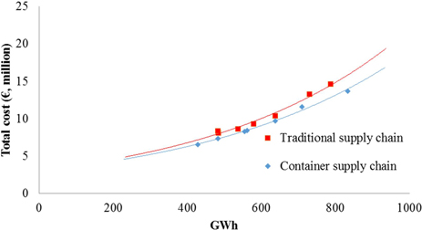
Fig. 11. Total cost (€, million) of traditional and container supply chains by trucks for forest chips (current dimensions).
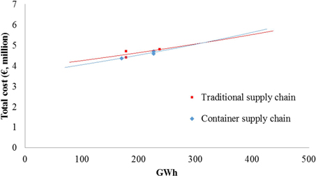
Fig. 12. Total cost (€, million) of traditional multimodal and container intermodal railway supply chains for forest chips (current dimensions).
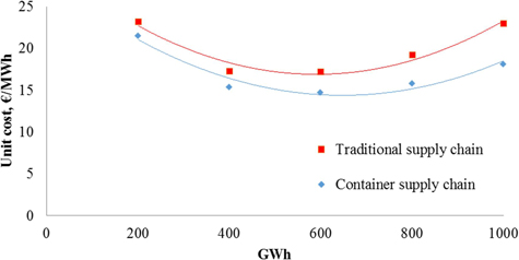
Fig. 13. Unit cost (€/MWh) of traditional and container supply chains by trucks for forest chips (current dimensions).
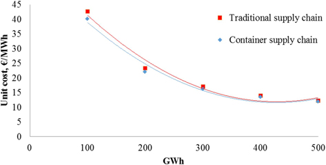
Fig. 14. Unit cost (€/MWh) of traditional multimodal and container intermodal railway supply chains for forest chips (current dimensions).
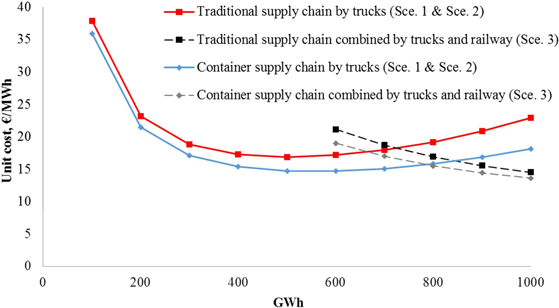
Fig. 15. Unit cost (€/MWh) of traditional and container supply chain scenarios for truck transportation (Sce. 1 & Sce. 2) and multimodal transportation (Sce. 3) for forest chips (current dimensions). The delivery amount of forest chips by trucks was kept constant (500 GWh) for multimodal supply chains (Sce. 3).
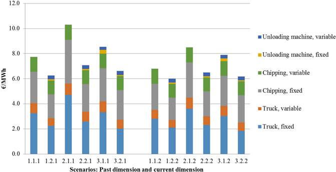
Fig. 16. Cost result (€/MWh) of simulation for truck transportation, chipping and the unloading machine in alternative scenarios (past and current dimension). Scenarios are presented in Table 1.
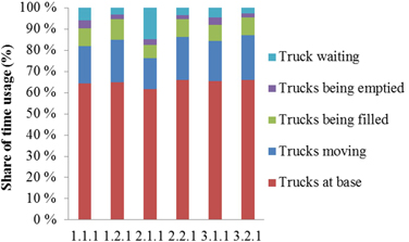
Fig. 17. Annual time usage of trucks in the scenarios (past dimension). Scenarios are presented in Table 1.
| Table 9. Average driving distances (in parentheses: maximum driving distance) by the trucks based on availability analysis for the target demand scenarios. | |||
| Distance, km | Sce. 1 | Sce. 2 | Sce. 3 |
| Logging residues | 61 (92) | 69 (103) | 59 (88) |
| Small-diameter energy wood | 81 (121) | 96 (144) | 71 (106) |
| Average | 71 (107) | 83 (124) | 65 (98) |