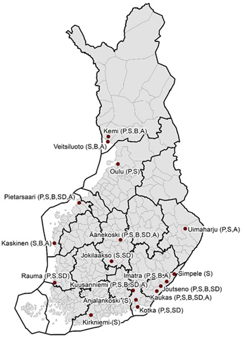
Fig. 1. Locations of the paper and pulp mills from which sample-based measurements were included in the green density prediction study material (P = pine, S = spruce, B = birch, SD = decayed spruce, A = aspen).
| Table 1. The number of observations by pulpwood assortments in the green density prediction study material. | ||||||||
| Pulpwood assortment | Total | Year | ||||||
| 2013 | 2014 | 2015 | 2016 | 2017 | 2018 | 2019 | ||
| Pine 1) | 20 299 | 3421 | 2488 | 4677 | 3699 | 2456 | 1867 | 1691 |
| Spruce 2) | 10 769 | 1120 | 1072 | 1344 | 1706 | 2015 | 1955 | 1557 |
| Spruce, decayed 3) | 2991 | 221 | 238 | 304 | 447 | 789 | 538 | 454 |
| Birch 4) | 17 423 | 2854 | 2455 | 3111 | 3027 | 2446 | 1852 | 1678 |
| Aspen 5) | 2293 | 281 | 222 | 215 | 365 | 522 | 385 | 303 |
| 1) Contain mainly Scots Pine (Pinus sylvestris); 2), 3) mainly Norway spruce (Picea abies); 4) mainly downy birch (Betula pubescens) or/and silver birch (Betula pendula); 5) mainly aspen (Populus tremula). | ||||||||
| Table 2. Green density (kg m–3) values and storage time of green density prediction study material by pulpwood assortments. | |||||||
| Pulpwood assortment | Number of observations | Green density, kg m–3 | Storage time, days | ||||
| Mean | Std | Median | Mean | Std | Median | ||
| Pine | 20 299 | 878.9 | 71.0 | 892 | 70 | 83 | 40 |
| Spruce | 10 769 | 845.7 | 64.3 | 854 | 38 | 48 | 21 |
| Spruce, decayed | 2991 | 731.6 | 56.4 | 732 | 43 | 56 | 26 |
| Birch | 17 423 | 868.3 | 65.9 | 881 | 70 | 79 | 40 |
| Aspen | 2293 | 804.4 | 60.2 | 809 | 50 | 57 | 29 |
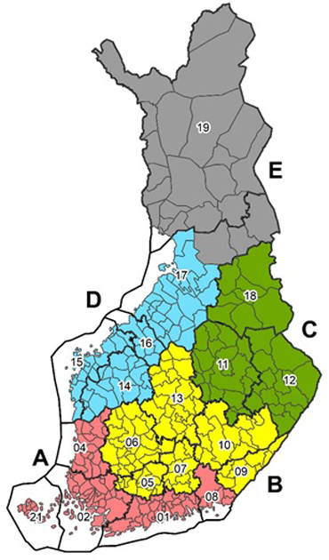
Fig. 2. Sub-areas (A–E) for the regional calibration used in green density MODELS 2.
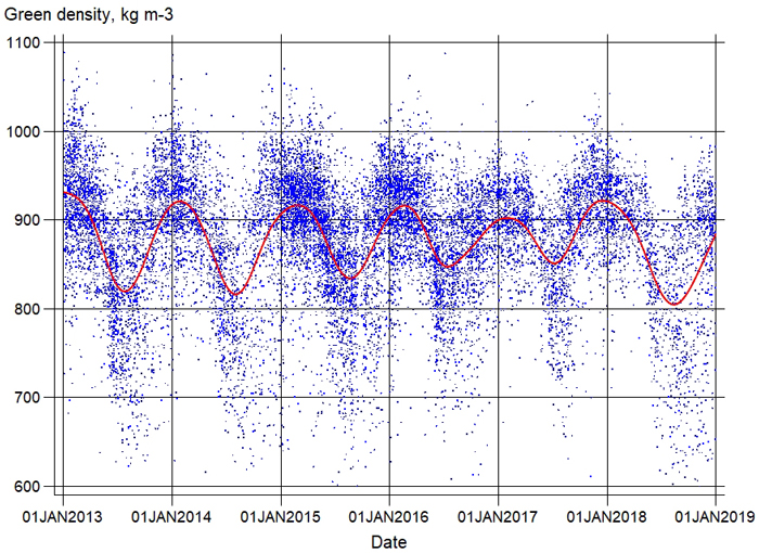
Fig. 3. Green density values of pine of the green density modeling data in 2013–2018. Red line indicates trimmed moving average.
| Table 3. Parameter estimates of models for green density (kg m–3) of the pulpwood assortments (MODELS 1). The standard error of the estimates is presented in parenthesis. | |||||
| Pine | Spruce | Spruce, decayed | Birch | Aspen | |
| Variable | Estimate | Estimate | Estimate | Estimate | Estimate |
| Intercept | 908.07 (3.753) | 865.05 (3.431) | 749.79 (6.566) | 931.56 (6.644) | 362.91 (113.98) |
| WEEK | –1.224 (0.466) | –4.078 (1.048) | |||
| WEEK>22 | 5.431 (1.176) | 2.085 (0.672) | |||
| WEEK2 | –0.061 (0.014) | 0.339 (0.068) | |||
| WEEK2>15 | 0.535 (0.098) | ||||
| WEEK2>20 | 0.194 (0.083) | ||||
| WEEK2>22 | 1.015 (0.172) | ||||
| WEEK3 | –0.0052 (0.001) | –0.01165 (0.002) | –0.0014 (0.0006) | ||
| STORAGE | –0.219 (0.043) | –0.307 (0.068) | –1.033 (0.080) | –0.733 (0.038) | –0.496 (0.092) |
| STORAGE>300 days | 0.284 (0.020) | 0.259 (0.107) | 0.245 (0.053) | 0.295 (0.021) | |
| STORAGENov-March | 0.264 (0.047) | 0.204 (0.075) | 0.686 (0.042) | ||
| STORAGEOct-Apr | 1.125 (0.073) | ||||
| STORAGEDec-March | 0.345 (0.104) | ||||
| STORAGEMay | –0.333 (0.087) | 0.445 (0.084) | |||
| STORAGEJune | –0.716 (0.094) | –1.268 (0.144) | 0.395 (0.104) | ||
| STORAGEJuly | –0.539 (0.109) | ||||
| TS | –0.157 (0.008) | –0.162 (0.015) | –0.034 (0.007) | –0.067 (0.010) | |
| TEMP | –0.532 (0.166) | –6.439 (1.189) | |||
| ln(TEMP+30) | 138.19 (33.746) | ||||
| TEMP3month | –0.791 (0.126) | –0.767 (0.290) | –0.765 (0.121) | ||
| TEMPmax20 | 0.550 (0.102) | 0.821 (0.201) | 0.433 (0.083) | ||
| ln(TEMPmax20 +1) | –4.081 (0.902) | ||||
| RAINFALL | 0.304 (0.022) | 0.126 (0.031) | 0.146 (0.011) | 0.258 (0.036) | |
| RAINFALL3month | –0.080 (0.010) | ||||
| RAINFALLwater | 0.247 (0.012) | ||||
| AREAE×MONTHFeb-May | 13.652 (1.838) | ||||
| AREAB×TS | 0.020 (0.002) | ||||
| AREAC×TS | 0.038 (0.007) | ||||
| AREAE×TS | –0.018 (0.004) | ||||
| var(wij) | 147.34 | 149.06 | 131.51 | 177.03 | 148.98 |
| corr(wij) | 0.843 | 0.785 | 0.915 | 0.882 | 0.793 |
| var(eijk) | |||||
| MONTHJan-May × STORAGE<1month | 1802.89 | 1725.79 | 2098.89 | 1118.45 | 1784.02 |
| MONTHJan-May × STORAGE>1month | 2512.92 | 2545.36 | 2067.21 | 1594.11 | 1895.57 |
| MONTHJune-Dec × STORAGE<1month | 2175.07 | 2318.61 | 2144.50 | 1574.23 | 1875.02 |
| MONTHJune-Dec × STORAGE>1month | 3357.90 | 3240.48 | 2671.54 | 1929.57 | 1980.89 |
| WEEK, delivery date of pulpwood at the mill expressed as week number (1–52); WEEK>15, dummy variable for wood delivered after week number 15 expressed as WEEK-15 (week); WEEK>20, dummy variable for wood delivered after week number 20 expressed as WEEK-20 (week); WEEK>22, dummy variable for wood delivered after week number 22 expressed as WEEK-22 (week); STORAGE, storage time of pulpwood (day); STORAGE>300, dummy variable for storage time of pulpwood exceeded >300 days (day); STORAGENov-March, dummy variable for storage time of pulpwood between November and March (day); STORAGEOct-Apr, dummy variable for storage time of pulpwood between October and April (day); STORAGEDec-March, dummy variable for storage time of pulpwood between December and March (day); STORAGEMay, dummy variable for storage time of pulpwood in May (day); STORAGEJune, dummy variable for storage time of pulpwood in June (day); STORAGEJuly, dummy variable for storage time of pulpwood in July (day); TS, temperature sum with a +5 °C threshold (dd); TEMP, average temperature of the storage time (°C); TEMP3month, average temperature of the last three months or whole storage time when storage time <3 months (°C); TEMPmax20, the number of storage days when maximum temperature of the day is >20 °C; RAINFALL, precipitation during the storage time (mm); RAINFALL3month, precipitation of the last three months or whole storage time when storage time <3 months (mm); RAINFALLwater, precipitation during the storage time when average temperature of the days is >0 °C (mm); MONTHFeb-May, dummy variable for delivery time between February and May (0.1); AREAB, dummy variable for sub-area B; AREAC, dummy variable for sub-area C; AREAE, dummy variable for sub-area E; var(wij), variance of random week effect; corr(wij), autocorrelation of the successive weeks, var(eijk) error variance of pulpwood group k; MONTHJan-May, MONTHJune-Dec, error variance of group k when delivery date is January–May or June–December, STORAGE<1month and STORAGE>1month, error variance of group k when storage time is less than or more than 1 month. | |||||
| Table 4. Relative root mean squared prediction errors (%) of green density calculated from the single parcels for four prediction methods: using the fixed part of the new models only (Fixed), correcting Fixed by the predicted week effect (Calibrated), using mill-specific trimmed moving averages of the last seven sample measurements (MOVING AVG), and using fixed green density factors (FGDF). | ||||
| Pulpwood assortment | rRMSE, % | |||
| Fixed | Calibrated | MOVING AVG | FGDF | |
| Pine | 6.70 | 6.30 | 7.91 | 8.89 |
| Spruce | 6.63 | 6.63 | 7.61 | 7.12 |
| Spruce, decayed | 6.06 | 5.98 | 7.25 | 6.86 |
| Birch | 5.23 | 4.79 | 6.45 | 6.63 |
| Aspen | 6.11 | 5.74 | 7.06 | 7.98 |
| Table 5. Relative root mean squared prediction errors (%) of green density calculated from weekly averages; using the fixed part of the new models only (Fixed), correcting Fixed by the predicted week effect (Calibrated), using mill-specific trimmed moving averages of the last seven sample measurements (MOVING AVG), and using fixed green density factors (FGDF). | ||||
| Pulpwood assortment | rRMSE, % | |||
| Tree species | Fixed | Calibrated | MOVING AVG | FGDF |
| Pine | 2.20 | 1.34 | 1.39 | 4.54 |
| Spruce | 1.40 | 1.22 | 1.51 | 2.64 |
| Spruce, decayed | 2.96 | 2.62 | 3.38 | 3.24 |
| Birch | 2.09 | 0.90 | 1.33 | 2.82 |
| Aspen | 4.05 | 3.40 | 4.99 | 5.48 |
| Table 6. Differences in the annual averages over the whole test data (year 2019) between the predicted and measured green densities (kg m–3) by pulpwood assortments; predictions both with fixed part of the model and after calibration, using the predicted week effects. | |||
| Pulpwood assortment | N | Prediction error Mean | |
| Fixed | Nationwide calibration | ||
| Pine | 1691 | –14.6 | –2.7 |
| Spruce | 1557 | –4.2 | –1.8 |
| Spruce, decayed | 454 | –3.6 | –1.1 |
| Birch | 1678 | –13.6 | –0.8 |
| Aspen | 303 | –15.7 | –7.4 |
| N, number of observations in test data (2019); Fixed, fixed predictions of the developed models; Nationwide calibration, predictions calibrated at national level. | |||
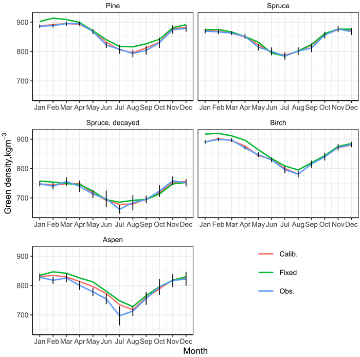
Fig. 4. Averages of observed (Obs.) and predicted (Fixed, Calib.) green density values in the test data (2019) by month. Fixed is fixed predictions. Calib. is the predictions obtained with the nationwide calibration.
| Table 7. Differences in the annual sub-area level averages over the whole test data (year 2019) between the predicted and measured green densities (kg m–3) by pulpwood assortments; predictions both with fixed part of the model and after calibration, using the predicted week effects. | ||||
| Sub-area | N | Prediction error Mean | ||
| Fixed | Nationwide calibration | Regional calibration | ||
| A | 193 | –17.3 | –7.0 | –8.4 |
| B | 826 | –18.3 | –5.7 | –4.1 |
| C | 38 | –16.0 | –3.8 | NA* |
| D | 506 | –16.3 | –4.5 | –6.2 |
| E | 128 | 19.8 | 31.3 | 8.3 |
| N, number of observations in test data (2019); Fixed, fixed predictions of the developed models; Nationwide calibration, predictions calibrated at national level; Regional calibration, predictions calibrated at reginal level. *Could not be estimated due to low number of observations. | ||||
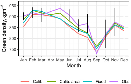
Fig. 5. Monthly averages of observed (Obs.) and predicted (Fixed, Calib. Calib_area) green density values in sub-area E (North Finland) in the test data (2019). Fixed is fixed predictions. Calib. is the predictions obtained with the nationwide calibration. Calib_area is the predictions obtained with the regional calibration.