| Table 1. Aboveground woody biomass (AGB) validation experiments comparing terrestrial laser scanned biomass estimates with destructively assessed biomass. Beam exit diameter and beam divergence from RIEGL Laser Measurement Systems GmbH (2020), Momo Takoudjou et al. (2017) and Faro Technologies Inc. (2009). The foliage column indicates if, at the time of scanning, needles or leaves were present. n: number of trees. Some authors have removed leaves from leaf-on point clouds prior to QSM generation. ‘Tree parts’ details which parts of the tree were compared between scans and destructive measurements. Full tree: all above ground parts, leafs excluded. In two cases, an upper branch diameter limit was used such that QSMs were pruned to the threshold diameter. The reported aggregated bias in aboveground biomass (AGB) estimate with TLS with respect to destructive values is shown in percentage. Volume estimates were obtained with SimpleTree a, TreeQSM b and voxelisation c (sensu Bienert et al. 2014). One case d compared full tree destructive AGB with >5 cm diameter TLS-derived AGB. | |||||||
| Reference | Scanner | Beam exit diameter and divergence (mm, mrad) | Foliage | n | Leaf stripping | Tree parts | Plot AGB bias |
| Calders et al. (2015) | RIEGL VZ-400 | 7, 0.35 | Leaf-on | 65 | No | Full tree | +9.68% b |
| Hackenberg et al. (2015a) | Z+F IMAGER 5010 | - | Leaf-off | 12 | No | Full tree | +2.42% a +19.6% b |
| Hackenberg et al. (2015a) | Z+F IMAGER 5010 | - | Leaf-on | 12 | Intensity thresholding + Eucl. Clustering | Full tree | +3.6% a –0.6% b |
| Hackenberg et al. (2015a) | Z+F IMAGER 5010 | - | Needle-on | 12 | Intensity thresholding + NN | Full tree | –17.0% a –4.6% b |
| Momo Takoudjou et al. (2017) | Leica C10 Scanstation | 4.5, 0 | Leaf-on | 61 | Manual | > 5 cm diameter | +5.2%a |
| Burt et al. (2021) | RIEGL VZ-400 | 7, 0.35 | Leaf-on | 4 | TLSeparation v1.2.1.5 | Full tree | –0.8% b |
| Gonzalez de Tanago et al. (2018) | RIEGL VZ-400 | 7, 0.35 | Leaf-on | 29 | No | > 10 cm diameter | –3.7%b |
| Kunz et al. (2017) | FARO Photon 120 | 3.3, 0.16 | Leaf-off | 24 | No | Full tree | –0.8% c –5.5% b –17.3% a |
| Thesis (Burt 2017) | RIEGL VZ-400 | 7, 0.35 | Leaf-off Leaf-on | 3 | No No | > 5 cm diameter | +3.7% b,d +26% b,d |
| Lau et al. (2019) | RIEGL VZ-400 | 7, 0.35 | Leaf-on | 26 | TLSeparation | Full tree | +2.9%b |
| Kükenbrink et al. (2021) | RIEGL VZ-1000 | 7, 0.35 | Almost leaf-off | 55 | Manual, few trees | Full tree | –9.5% |
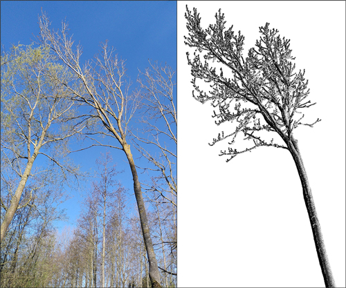
Fig. 1. Photograph and point cloud of common ash #2. (left) Ash #2 before felling (on the foreground). (right) Point cloud visualisation of the same tree from the same upward looking perspective as the photographer.
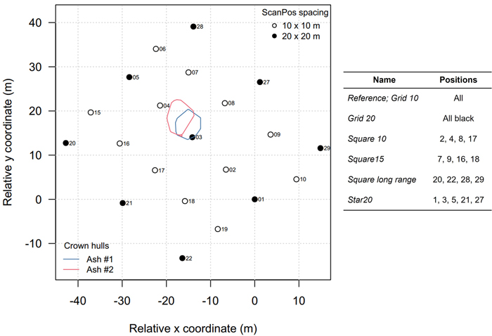
Fig. 2. Map of the scanning pattern. The locations of the harvested ash trees are depicted as vertical projections of their crown hulls. The scan positions of the modulations are shown on the right.
| Table 2. The 14 point cloud modulations constructed for each of the two ash trees. | ||
| Modulation type | Name | Description |
| Reference | Grid 10 | 10 × 10 m square grid, MSA1, filtered for deviation and reflectance |
| Scan pattern | Grid 20 Square 10 Square 15 Square longrange Star | See Fig. 3 and text |
| Range | Range20 … Range 35 | Points further away than respectively 20, 22.5, 25, 30, 35 m removed |
| Unfiltered | Unfiltered | Same as Reference but without filtering |
| Fuzz filtering | Fuzz | Same as Reference but with additional Fuzz filtering |
| Multi-station adjustment module 2 | MSA2 | Same as Reference but MSA 2 instead of MSA1 |
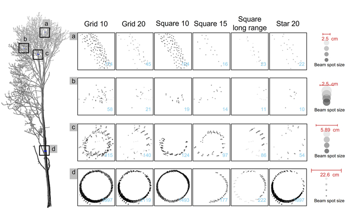
Fig. 3. Examples of common ash branch segment point clouds under a variation of scan position layouts. See Fig. 2 for a description of scan position variations. Segments have a zenith point of view. Points coloured on beam spot size; red bar shows the true-to-scale manually measured branch diameters at each location and the true-to-scale beam spot sizes. In blue the number of points per segment is shown. The manual diameters were 25, 25, 58.9, and 226 mm each segment. View larger in new window/tab.
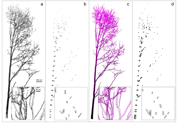
Fig. 4. TLS point cloud and QSM reconstruction of common ash #2. Bottom: magnification of branches in the upper part of the crown (location indicated by the parallelogram – direction of view indicated by the arrow in panel c). (a) Full point cloud. (b) Manually segmented 10 cm long branch sections. (c) Full QSM of the tree (coloured by z-coordinate value). (d) Individual QSM cylinders that have been successfully matched with the manual measurements. View larger in new window/tab.
| Table 3. General characteristics of the harvested common ash trees and overview of destructive tree mass measurements, conversion factors and converted volumes for two ash trees. The results are divided into diameter classes of the sampled material. ‘Full tree’ marks either the total mass or volume per tree, or the weighted wood properties. Additionally, the compartmentalised volumes of the optimised reference modulation quantitative structure model (QSM) are added. AGB: aboveground biomass. FWD: Fresh wood density. ρ: Basic wood density. DMC: dry matter content. We used ‘tree length’ rather than tree height because this was measured on the felled tree. | |||||||||||
| DBH (cm) | Tree length (cm) | Scan & harvest date | Fresh mass (kg) | Volume (L) | QSM (L) | AGB (kg) | FWD (kg m–3) | ρ (kg m–3) | DMC (kg kg–1) | ||
| Ash #1 | 27.4 | 1957 | 19/03 & 03/04 2020 | Full tree | 646.5 | 731.9 | 1114 | 421.4 | 883 | 576 | 0.652 |
| >10 cm | 456.5 | 506.7 | 542 | 300.5 | 901 | 593 | 0.658 | ||||
| 7–10 cm | 34.0 | 39.4 | 60.6 | 22.7 | 864 | 577 | 0.668 | ||||
| 5–7 cm | 44.9 | 53.4 | 61.8 | 30.2 | 841 | 565 | 0.672 | ||||
| 2.5–5 cm | 53.6 | 62.8 | 234 | 34.6 | 855 | 551 | 0.645 | ||||
| 0–2.5 cm | 57.4 | 69.5 | 216 | 33.4 | 826 | 480 | 0.581 | ||||
| Ash #2 | 29.4 | 1905 | 19/03 & 07/04 2020 | Full tree | 713.1 | 868.2 | 1201 | 461.0 | 821 | 531 | 0.647 |
| >10 cm | 509.0 | 620.6 | 643 | 332.8 | 820 | 536 | 0.654 | ||||
| 7–10 cm | 34.9 | 41.3 | 58.9 | 22.9 | 844 | 555 | 0.658 | ||||
| 5–7 cm | 34.3 | 40.8 | 67.4 | 22.5 | 840 | 551 | 0.655 | ||||
| 2.5–5 cm | 70.2 | 85.4 | 256 | 44.4 | 823 | 520 | 0.632 | ||||
| 0–2.5 cm | 64.7 | 80.0 | 176 | 38.5 | 808 | 481 | 0.595 | ||||
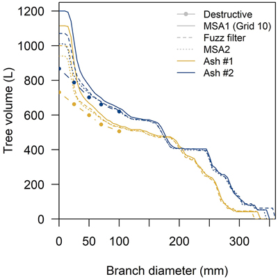
Fig. 5. QSM and destructive cumulative volume repartitioning in common ash based on branch diameter sizes. Grey/white bands indicate the branch diameter classes used in the destructive measurements. QSM volumes obtained with the Grid 10 modulation (coregistered using Multi-Station Adjustment 1 (MSA1)), a fuzz filtered and MSA2 point cloud.
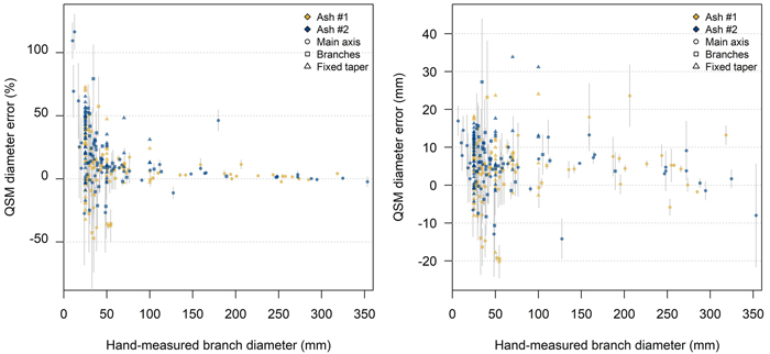
Fig. 6. Relative (left) and absolute (right) error in the diameter of common ash QSM cylinders from the reference point cloud ‘Grid 10’ with respect to manually measured branch diameters. Comparison of hand-measured branch diameters and diameters from five QSM reconstruction (mean and standard deviation as grey whiskers). Light-grey/white bands indicate branch diameter classes. The fixed taper measurements are located at the thresholds of the diameter classes. For reasons of clarity, here no standard deviation whiskers are plotted. For visualisation purposes one outlier (error = 257% and hand-measured diameter = 3.3 mm) is not within the plotting frame. View larger in new window/tab.
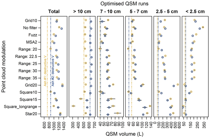
Fig. 7. Comparison of the QSM volume against destructively measured volume (dashed line) in 5 diameter classes for 12 different point cloud modulations, the fuzz filtered point cloud and the Multi-Station Adjustment 2 coregistration in two common ash trees. QSM volume was extracted as the mean (points) and standard deviation (black whiskers) of five models with optimal input parameters. See Fig. 2 for a description of the scanning patterns.
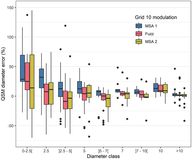
Fig. 8. Common ash branch diameter error of QSMs with respect to manually measured branches in branch diameter classes. Positive values indicate an overestimation of QSM diameters with respect to manual measurements. Three modulations were compared: the ‘Grid 10’ reference modulation using the standard Multi-Station Adjustment 1 (MSA1) algorithm, the fuzz filtered point cloud and the MSA2 registered point cloud. For visualisation purposes one outlier (error = 257% and diameter class <2.5 mm; MSA1) is not within the plotting frame. Box line represents median value, the upper and lower hinges represent the 25th and 75th percentile and the whiskers extend to the min/max values, except if min/max values are further than 1.5 times the interquartile range (these points are outliers: black dots).
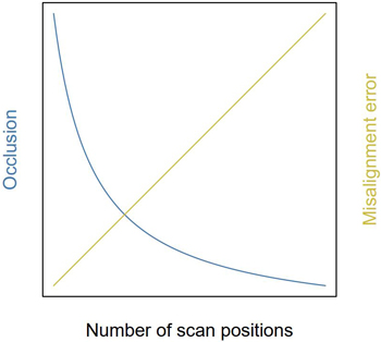
Fig. 9. Conceptual figure of the trade-off for optimal amount of scan positions. Theoretical implication of the number of scan positions on point cloud quality. This trade-off in amount of scan position balances the effects of occlusion and misalignment errors due to coregistration and wind.
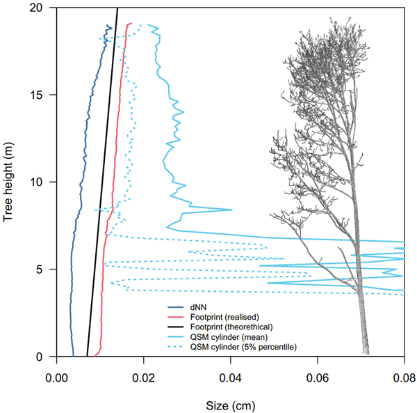
Fig. 10. Sizes of laser beam footprint, QSM cylinders and nearest neighbour distances of common ash #1 in function of tree height. dNN: the mean distance to the closest neighbouring point in 10 cm z-slices. The laser beam footprint diameter size was calculated from the ranging distance to the scanner. The realised footprint was inferred from the range of each point in the point cloud and averaged in 10 cm z-slices. The theoretical footprint was simulated from a scanner position at ground level. ‘QSM cylinder’ are the average and 5% percentile of QSM cylinder diameters in 20 cm z-slices.