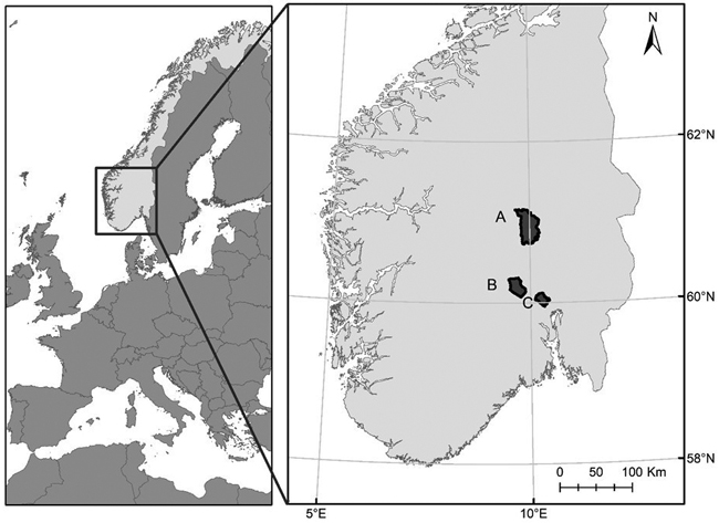
Fig. 1. Location of the three districts used in the study: Nordre Land (A), Krødsherad (B), and Hole (C).
| Table 1. Overview of the districts (A, B, and C) and their measured plots used in the study at two points in time (T1 and T2). | |||||||||||||||
| Training plot T1 | Training plot T2 | Validation plot T2 | |||||||||||||
| District | Elev. | Year | n | ps | P | Year | n | ps | P | n | ps | P | |||
| A | 140–900 | 2003 | 193 | 250 | 0.73 | 2017 | 170 | 250 | 0.64 | 25 | 1000 | 0.28 | |||
| B | 130–660 | 2001 | 74 | 232.9 | 0.39 | 2016/17 | 75 | 232.9 | 0.35 | 43 | 3721 | 0.44 | |||
| C | 240–480 | 2005 | 78 | 250 | 1 | 2017 | 43 | 250 | 1 | 22 | 1000 | 1 | |||
| Elev. = elevation above sea level (m); n = number of plots; ps = plot size (m2); P = proportion of spruce-dominated plots. | |||||||||||||||
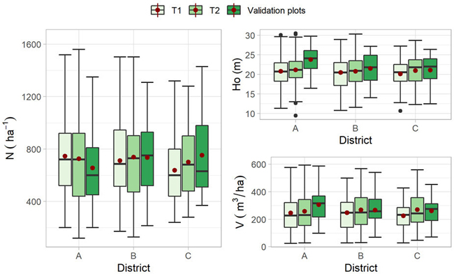
Fig. 2. Box plots showing the distribution of the field plot attributes per district (dominant heigh (Ho), volume (V), and stem number (N)) for the training plots measured at two points in time (T1 and T2) and the validation plots measured at T2. The mean value is indicated with a red dot.
| Table 2. Summary of ALS instrument specifications and flight acquisition parameter settings for the different districts (A, B and C). | ||||||
| District | year | Instrument | Mean flying altitude (m) | Pulse repetition frequency (kHz) | Scanning frequency (Hz) | Mean point density (pts m–2) |
| First acquisition (T1) | ||||||
| A | 2003 | Optech ALTM 1233 | 800 | 33 | 40 | 1 |
| B | 2001 | Optech ALTM 1210 | 650 | 10 | 30 | 1 |
| C | 2005 | Optech ALTM 3100 | 2000 | 50 | 38 | 1 |
| Second acquisition (T2) | ||||||
| A | 2016 | Riegl LMS Q-1560 | 2900 | 400 | 100 | 4 |
| B | 2016 | Riegl LMS Q-1560 | 1300 | 534 | 115 | 12 |
| C | 2016 | Riegl LMS Q-1560 | 1300 | 534 | 115 | 10 |
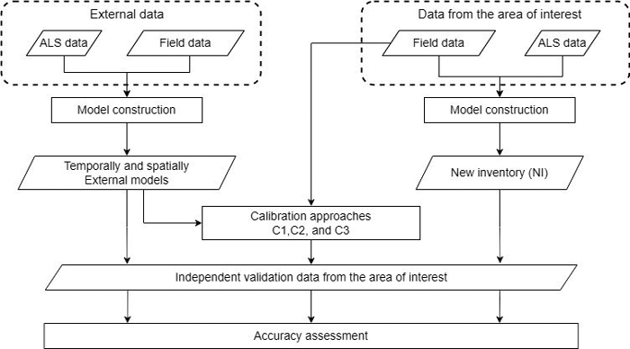
Fig. 3. Flowchart showing the main analysis of the methodology to calibrate forest attribute predictions from external models.
| Table 3. Results of the two-sample Kolmogorov-Smirnov test between the training field plots measured at two points in time (T1 and T2) and the validation plots measured at T2 in the three districts (A, B and C). | ||||||||||
| Validation district A (T2) | Validation district B (T2) | Validation district C (T2) | ||||||||
| District | Statistic | H | V | N | H | V | N | H | V | N |
| A (T1) | D | 0.39 | 0.28 | 0.22 | ||||||
| p-value | 0.002 | 0.04 | 0.22 | |||||||
| A (T2) | D | 0.36 | 0.24 | 0.26 | 0.14 | 0.17 | 0.12 | 0.13 | 0.20 | 0.18 |
| p-value | 0.005 | 0.14 | 0.10 | 0.43 | 0.22 | 0.69 | 0.86 | 0.41 | 0.55 | |
| B (T1) | D | 0.19 | 0.21 | 0.21 | ||||||
| p-value | 0.25 | 0.14 | 0.20 | |||||||
| B (T2) | D | 0.17 | 0.15 | 0.10 | ||||||
| p-value | 0.37 | 0.51 | 0.93 | |||||||
| C (T1) | D | 0.22 | 0.28 | 0.19 | ||||||
| p-value | 0.38 | 0.14 | 0.52 | |||||||
| C (T2) | D | 0.08 | 0.24 | 0.15 | ||||||
| p-value | 1 | 0.37 | 0.88 | |||||||
| Table 4. Selected predictors and validation results for temporally and spatially externally models for Ho, V and N. RMSE% and relative mean difference of predictions (MD%) with corresponding 95% confidence intervals (CIRMSE, CIMD), and error model parameters (λ0, λ1, and σεm) were calculated after application of the models on validation datasets from districts A, B, and C. | |||||||||
| Predictors* | RMSE% | CIRMSE | MD% | CIMD | λ0 | λ1 | σεm | ||
| Temporal | |||||||||
| A | Ho | H90, D0 | 8.3 | 5.8, 10.9 | –2.0 | –5.1, 1 | 7.0 | 0.7 | 1.5 |
| V | H70, D0 | 22.6 | 16.1, 29.1 | 9.1 | –0.1, 17.4 | 90.8 | 0.8 | 62.0 | |
| N | Hmax, D0, D9 | 25.8 | 19.0, 33.1 | 2.1 | –8.4, 12.4 | 267.5 | 0.6 | 135.0 | |
| B | Ho | H90, D5 | 5.1 | 3.7,6.5 | 0.4 | –1.2, 1.9 | 4.1 | 0.8 | 0.9 |
| V | H80, D0 | 15.6 | 9.8, 22.0 | 5.1 | 0.6, 9.6 | 49.7 | 0.9 | 37.0 | |
| N | H80, D1 | 26.8 | 19.2, 34.8 | –7.1 | –13.9, –0.1 | 320.8 | 0.5 | 125.8 | |
| C | Ho | H90, D0, D7 | 4.5 | 3.3, 5.8 | 2.0 | 0.3, 3.8 | 2.3 | 0.9 | 0.8 |
| V | H40, D4 | 19.0 | 11.7, 26.9 | 5.9 | –2.2, 14 | 52.5 | 0.9 | 44.4 | |
| N | H90, D4 | 25.1 | 17.5, 34 | –9.9 | –18.1, –1.7 | 285.3 | 0.5 | 100.3 | |
| Spatial | |||||||||
| B | Ho | H90 | 5.3 | 3.8, 6.7 | 1.5 | –0.1, 3.1 | 5.2 | 0.8 | 0.7 |
| V | H90, D0, D8 | 21.2 | 14.1, 28.9 | 11.4 | 6.5, 16.6 | 1.7 | 1.1 | 46.6 | |
| N | Hmax, H30, D0 | 26.0 | 17.4, 34.4 | 12.5 | 4.3, 20.1 | 266.8 | 0.8 | 158.8 | |
| C | Ho | H90 | 5.0 | 3.5, 6.6 | –0.5 | –2.3, 2.0 | 4.1 | 0.8 | 0.8 |
| V | H90, D0, D8 | 19.8 | 10.5, 29.1 | 4.7 | –3.3, 12.4 | 48.9 | 0.9 | 46.0 | |
| N | Hmax, H30, D0 | 26.3 | 18.5, 34.6 | 15.5 | 5.5, 25.4 | 291.7 | 0.8 | 145.9 | |
| * H30, H40, H70, H80 and H90 = 30, 40, 70, 80 and 90 percentiles of the laser canopy heights; Hmax = maximum laser canopy height; D0, D1, … D9 = canopy densities corresponding to the proportions of laser returns above each bin # 0, 1, … 9, respectively, to total number of returns (see text). | |||||||||
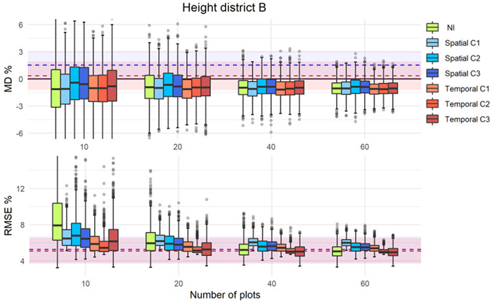
Fig. 4. MD% and RMSE% distributions from 1000 iterations in simulations of different calibration approaches (as boxplots) using external prediction models of dominant height in district B. The MD% (upper panel) and RMSE% (lower panel) of uncalibrated external predictions are displayed with dashed lines (blue = spatial, red = temporal) with corresponding confidence intervals displayed as colored areas around the respective lines.
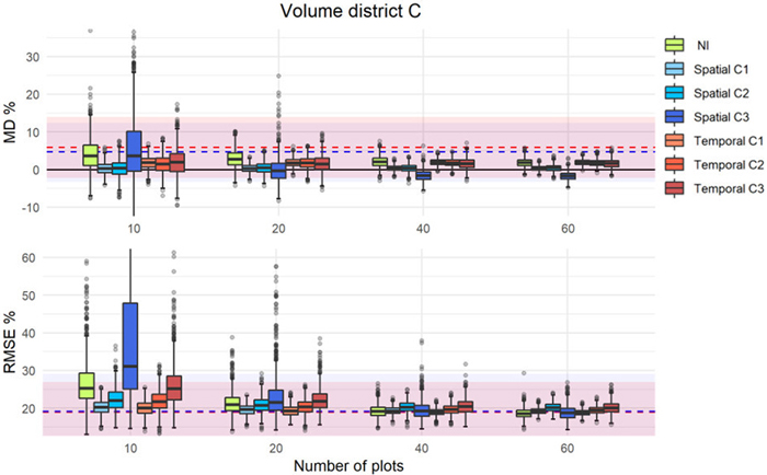
Fig. 5. MD% (upper) and RMSE% (lower) distributions from 1000 iterations in simulations of different calibration approaches (as boxplots) using external prediction models of volume in district C. The uncalibrated external predictions are displayed with dashed lines (blue = spatial, red = temporal) with the corresponding confidence intervals as colored areas around the respective lines.
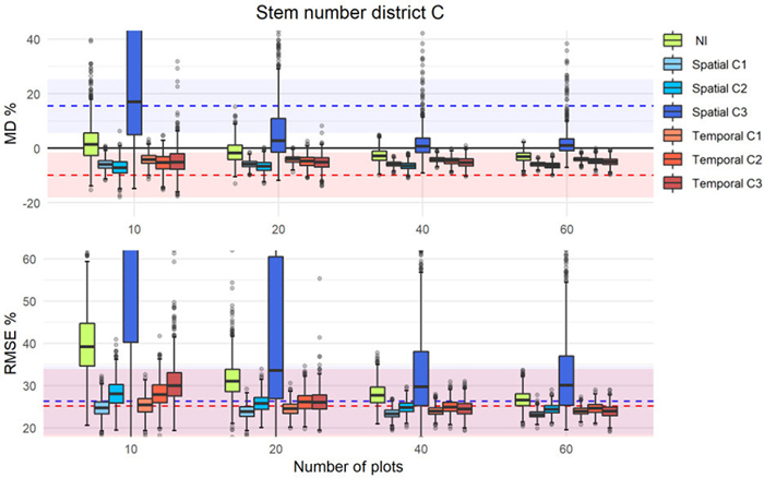
Fig. 6. MD% and RMSE% distributions from 1000 iterations in simulations of different calibration approaches (as boxplots) using external prediction models of stem number in district C. The MD% (upper panel) and RMSE% (lower panel) of uncalibrated external predictions are displayed with dashed lines (blue = spatial, red = temporal) with corresponding confidence intervals displayed as colored areas around the respective lines.
| Table 5. Median values of RMSE%, MD%, λ0, λ1, and σεm after 1000 iterations of applying the different calibration approaches (C1, C2, and C3) using 20 calibration plots, and the new inventory where the prediction models were created with 60 plots (NI60) for each district (A, B, and C). | ||||||||||||||||
| Ho | V | N | ||||||||||||||
| A | NI60 | 8.4 | –1.5 | 8.2 | 0.6 | 1.5 | 22.8 | 4.1 | 75.0 | 0.8 | 67.7 | 27.2 | 11.8 | 235.9 | 0.8 | 148.9 |
| Temporal C1 | 8.5 | –1.5 | 8.0 | 0.7 | 1.5 | 22.5 | 3.7 | 88.0 | 0.8 | 63.0 | 29.4 | 6.2 | 319.6 | 0.6 | 150.4 | |
| Temporal C2 | 9.3 | –1.8 | 8.3 | 0.6 | 1.7 | 25.3 | 6.3 | 64.9 | 0.9 | 76.6 | 30.4 | 5.5 | 301.55 | 0.6 | 163.3 | |
| Temporal C3 | 9.0 | –1.6 | 8.1 | 0.6 | 1.6 | 23.9 | 4.6 | 56.3 | 0.89 | 73.4 | 31.9 | 11.2 | 227.9 | 0.8 | 185.8 | |
| B | NI60 | 5.1 | –1.1 | 2.9 | 0.9 | 0.9 | 19.4 | 7.6 | 33.6 | 1.0 | 45.7 | 26.0 | 7.2 | 210.8 | 0.8 | 177.3 |
| Temporal C1 | 5.6 | –1.1 | 4.0 | 0.8 | 0.9 | 17.2 | 6.6 | 48.6 | 0.9 | 38.8 | 24.9 | 5.2 | 293.7 | 0.7 | 149.5 | |
| Temporal C2 | 5.1 | –0.9 | 2.8 | 0.9 | 0.9 | 17.2 | 6.7 | 31.4 | 1.0 | 40.7 | 26.7 | 5.3 | 302.6 | 0.7 | 163.0 | |
| Temporal C3 | 5.3 | –0.9 | 2.5 | 0.9 | 0.9 | 18.8 | 6.8 | 31.3 | 1.0 | 44.1 | 26.4 | 5.4 | 262.0 | 0.7 | 168.5 | |
| Spatial C1 | 6.2 | –1.0 | 4.5 | 0.8 | 1.0 | 19.5 | 6.7 | 13.0 | 1.0 | 47.2 | 22.9 | 4.9 | 209.2 | 0.8 | 153.4 | |
| Spatial C2 | 5.9 | –0.7 | 3.0 | 0.9 | 1.0 | 18.6 | 6.2 | 29.9 | 1.0 | 43.8 | 24.0 | 4.0 | 189.6 | 0.8 | 162.7 | |
| Spatial C3 | 5.8 | –0.8 | 3.3 | 0.8 | 1.0 | 22.0 | 7.5 | 21.1 | 1.0 | 52.1 | 25.7 | 4.9 | 184.2 | 0.8 | 175.6 | |
| C | NI60 | 4.3 | 0.3 | 1.9 | 0.9 | 0.9 | 18.5 | 1.8 | 29.0 | 0.9 | 46.9 | 26.5 | –3.1 | 284.6 | 0.6 | 154.8 |
| Temporal C1 | 4.2 | –0.2 | 2.2 | 0.9 | 0.8 | 19.2 | 1.8 | 51.4 | 0.8 | 45.8 | 24.6 | –4.1 | 313.8 | 0.5 | 119.7 | |
| Temporal C2 | 4.2 | –0.2 | 1.4 | 0.9 | 0.9 | 20.3 | 1.8 | 38.2 | 0.9 | 50.4 | 26.1 | –4.8 | 304.9 | 0.5 | 135.7 | |
| Temporal C3 | 4.4 | –0.0 | 1.3 | 0.9 | 0.9 | 21.8 | 1.5 | 32.5 | 0.9 | 54.8 | 26.1 | –5.1 | 273.0 | 0.6 | 145.2 | |
| Spatial C1 | 5.2 | 0.1 | 4.2 | 0.8 | 0.8 | 19.6 | 0.3 | 48.0 | 0.8 | 47.2 | 23.9 | –5.9 | 246.2 | 0.6 | 131.0 | |
| Spatial C2 | 4.7 | 0.2 | 2.0 | 0.9 | 0.9 | 20.8 | 0.4 | 35.6 | 0.9 | 51.9 | 25.8 | –6.6 | 256.7 | 0.6 | 141.8 | |
| Spatial C3 | 4.9 | 0.2 | 2.1 | 0.9 | 1.0 | 21.5 | –0.4 | 29.3 | 0.9 | 54.0 | 33.6 | 2.7 | 276.5 | 0.7 | 223.5 | |