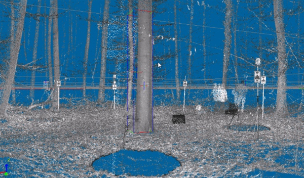
Fig. 1. Scan output showing a targeted beech. This scan was performed from four different directions.
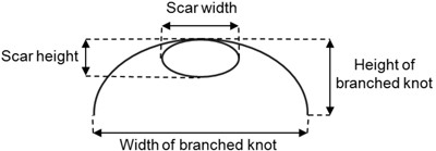
Fig. 2. Parameters measured at each bark characteristic.
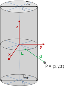
Fig. 3. New coordinate system {L,z,d} with cylinders as a basis to evaluate height differences with respect to the bark surface. Each point P of the laser scanning image can be defined in 3D space either in a Cartesian coordinate system by {x,y,z} or by the set {L,z,d} linked to the virtual cylinders describing a simplified tree stem surface. The axis of the cylinder is given by a pair of points ru and rd. Diameters of the top and bottom areas of the cylinder are denoted as Du and Dd.
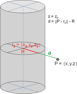
Fig. 4. Illustration of parameter d as the distance from the cylinder surface to point P.
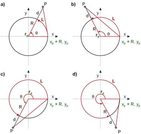
Fig. 5. Arc length L dependent on the position of P in the x-y coordinate system.
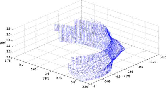
Fig. 6. The point cloud characterizing the user defined bark feature in 3D modus of the laser scanning image (conventional x,y,z system).
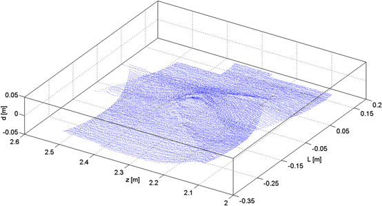
Fig. 7. Transformed 3D point cloud in the L,z,d coordinate system.
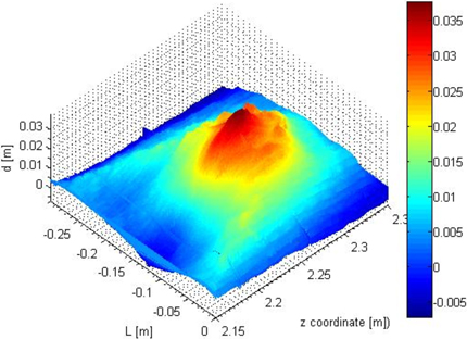
Fig. 8. The surface of a portion of a stem obtained by interpolation of the 3D point cloud is shown from an arbitrary point of view. The lower regions denoted in blue are below or even with the approximated stem surface. Yellow and red represent regions considerably higher than the surface of the stem approximated by cylinders.
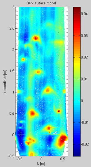
Fig. 9. Numerical reconstruction of the tree stem surface. By applying a coordinate transformation the stem of a tree is projected into a new coordinate system with z as the height above or below the scanner axis and L as the distance around the stem rectangular to the z-axis. The third dimension, the distance above or below the approximated cylinder surface, i.e. distance parameter d, is represented by colors ranging from blue (below or even with the cylinder surface) to red (points high above the cylinder surface).
| Table 1. Comparison of scars and branched knots measured manually and by use of TLS data. The trees taken into account were denoted V, W, and Y. As the logs were cut in parts, they were numbered V1, V2, W1, W2, Y1, and Y2. Each characteristic measured manually was then numbered beginning with the first measurement. The name of the characteristic indicates the log part it was found on, e.g. V1_1 means first characteristic on the first log of tree V. | ||||||||
| Scar number | Scar width [cm] | Scar height [cm] | Width of branched knot [cm] | Height of branched knot [cm] | ||||
| Manually | By TLS data | Manually | By TLS data | Manually | By TLS data | Manually | By TLS data | |
| V1_1 | 8.4 | 2.34 a) | 2.0 | 2.87 a) | 37.0 | 35.40 a) | 2.2 | 2.75 a) |
| V1_7 | 9.9 | 6.18 a) | 3.8 | 3.06 a) | 37.5 | 25.66 a) | 8.0 | 4.68 a) |
| V1_15 | 8.3 | 6.89 a) | 2.2 | 2.01 a) | 27.0 | 26.62 a) | 2.2 | 2.01 a) |
| V2_2 | 10.0 c) | 10.80 a) | 3.1 | 3.53 a) | --- | --- | 3.1 | --- |
| V2_6 | 12.0 | 7.15 b) | 11.0 | 12.47 b) | 57.0 | 16.26 b) | 16.0 | 21.34 b) |
| V2_12 | 6.7 | 8.05 a) | 4.8 | 4.64 a) | 34.2 | 30.70 a) | 8.7 | 7.03 a) |
| W1_3 | 13.5 | 13.44 b) | 4.0 | 3.74 b) | 37.5 | 38.54 b) | 6.5 | 4.67 b) |
| W1_6 | 6.2 | 4.03 b) | 2.0 | 1.58 b) | 25.0 | 21.29 b) | 3.0 | 3.52 b) |
| W1_10 | 4.0 | 4.14 a) | 2.8 | 2.92 a) | 19.0 | 7.79 a) | 7.0 | 5.65 a) |
| W2_11 | 5.4 | 5.58 a) | 6.2 | 6.18 a) | 36.0 | 13.82 a) | 18.8 | 11.35 a) |
| W2_15 | 4.5 | 4.45 a) | 5.0 | 5.82 a) | 27.0 | 17.30 a) | 21.0 | 14.80 a) |
| W2_16 | 6.0 | 5.15 a) | 6.2 | 5.91 a) | 28.0 | 22.20 a) | 18.0 | 16.60 a) |
| Y1_1 | 6.0 | 6.47 a) | 2.3 | 3.15 a) | 17.0 | 15.20 a) | 3.7 | 4.10 a) |
| Y1_2 | 10.5 | 12.68 a) | 3.7 | 4.23 a) | 40.5 | 34.20 a) | 6.8 | 6.20 a) |
| Y1_3 | 14.5 | 11.11 a) | 2.7 | 2.36 a) | 30.0 | 26.44 a) | 5.0 | 2.36 a) |
| Y2_3 | 9.6 | 7.57 a) | 3.5 | 3.91 a) | 27.0 | 29.90 a) | 4.9 | 4.90 a) |
| Y2_23 | 18.2 | 11.14 b) | 4.2 | 5.06 b) | 43.0 | 43.22 b) | 8.5 | 10.34 b) |
| Y2_27 | 14.3 | 10.48 b) | 8.3 | 8.17 b) | 35.0 | 36.33 b) | 14.0 | 11.88 b) |
| a) TLS measurements were performed by intensity data. b) TLS measurements were performed by use of the bark surface model. c) This result is not reliable due to the geometry of the intensity data. | ||||||||
| Table 2. Differences between the manual measurements on the felled tree and the measurements of the scars and branched knots by use of TLS data. The trees taken into account were denoted V, W, and Y. As the logs were cut in parts, they were numbered V1, V2, W1, W2, Y1, and Y2. Each characteristic measured manually was then numbered beginning with the first measurement. The name of the characteristic indicates the log part it was found on, e.g. V1_1 means first characteristic on the first log of tree V. | ||||||||
| Scar number | Scar width | Scar height | Width of branched knot | Height of branched knot | ||||
| Manual meas. [cm] | Difference [cm] | Manual meas. [cm] | Difference [cm] | Manual meas. [cm] | Difference [cm] | Manual meas. [cm] | Difference [cm] | |
| V1_1 | 8.4 | 6.06 | 2.0 | –0.87 | 37.0 | 1.60 | 2.2 | –0.55 |
| V1_7 | 9.9 | 3.72 | 3.8 | 0.74 | 37.5 | 11.84 | 8.0 | 3.32 |
| V1_15 | 8.3 | 1.41 | 2.2 | 0.19 | 27.0 | 0.38 | 2.2 | 0.19 |
| V2_2 | 10.0 | –0.80 | 3.1 | –0.43 | 0.00 | 3.1 | 3.10 | |
| V2_6 | 12.0 | 4.85 | 11.0 | –1.47 | 57.0 | 40.74 | 16.0 | –5.34 |
| V2_12 | 6.7 | –1.35 | 4.8 | 0.16 | 34.2 | 3.50 | 8.7 | 1.67 |
| W1_3 | 13.5 | 0.06 | 4.0 | 0.26 | 37.5 | –1.04 | 6.5 | 1.83 |
| W1_6 | 6.2 | 2.17 | 2.0 | 0.42 | 25.0 | 3.71 | 3.0 | –0.52 |
| W1_10 | 4.0 | –0.14 | 2.8 | –0.12 | 19.0 | 11.21 | 7.0 | 1.35 |
| W2_11 | 5.4 | –0.18 | 6.2 | 0.02 | 36.0 | 22.18 | 18.8 | 7.45 |
| W2_15 | 4.5 | 0.05 | 5.0 | –0.82 | 27.0 | 9.70 | 21.0 | 6.20 |
| W2_16 | 6.0 | 0.85 | 6.2 | 0.29 | 28.0 | 5.80 | 18.0 | 1.40 |
| Y1_1 | 6.0 | –0.47 | 2.3 | –0.85 | 17.0 | 1.80 | 3.7 | –0.40 |
| Y1_2 | 10.5 | –2.18 | 3.7 | –0.53 | 40.5 | 6.30 | 6.8 | 0.60 |
| Y1_3 | 14.5 | 3.39 | 2.7 | 0.34 | 30.0 | 3.56 | 5.0 | 2.64 |
| Y2_3 | 9.6 | 2.03 | 3.5 | –0.41 | 27.0 | –2.90 | 4.9 | 0.00 |
| Y2_23 | 18.2 | 7.06 | 4.2 | –0.86 | 43.0 | –0.22 | 8.5 | –1.84 |
| Y2_27 | 14.3 | 3.82 | 8.3 | 0.13 | 35.0 | –1.33 | 14.0 | 2.12 |
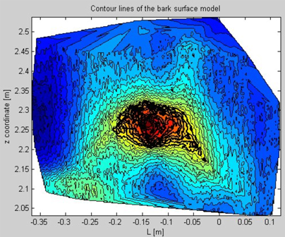
Fig. 10. Assembly of contour lines above a user-defined threshold. These lines are indicated by solid black lines.
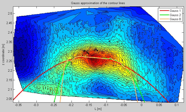
Fig. 11. Gaussian approximation of a bark characteristic with modifying degrees (1 = red, 2 = green, 8 = brown).
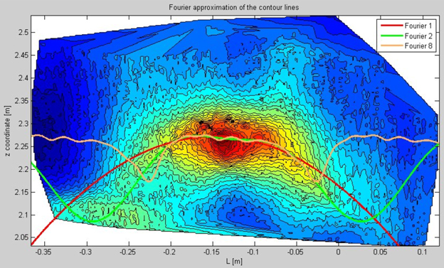
Fig. 12. Fourier approximation of a bark characteristic with modifying degrees (1 = red, 2 = green, 8 = brown).