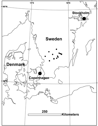
Fig. 1. Map of Southern Sweden showing the location of the surveyed stands.
| Table 1. Description of the environmental variables used in the statistical analyses. The variables are: Total basal area per ha (Bas tot); Stems per ha (Stems); Basal area per ha for aspen (Bas asp); Stand height (Height); Total number of living or dead retained trees > 10 cm DBH within 40 m of the four sample points (Ret tree); Number of thinned respectively unthinned stands (Thin); Total number of woody species (Tree spec); Tree evenness, the Shannon’s diversity index of the tree species composition divided by the log of the number of tree species (Tree even); % developed land within a 500 m radius (Devel); % agricultural land within a 500 m radius (Agric); % wetlands within a 500 m radius (Wetl); Volume coniferous trees per ha within a 500 m radius (Conif); Volume deciduous trees per ha within a 500 m radius (Decid). |
| | Spruce stands | Aspen stands |
| Mean | SD | Count | Mean | SD | Count |
| Bas tot (m2 ha–1) | 1.6 | 1.1 | | 3.2 | 1.7 | |
| Stems (no ha–1) | 9241 | 6181 | | 10882 | 5748 | |
| Bas asp (m2 ha–1) | 0.0 | 0.0 | | 1.1 | 0.5 | |
| Height (m) | 3.4 | 1.1 | | 5.2 | 0.8 | |
| Ret tree (no.) | 7 | 8 | | 3 | 3 | |
| Thin | Unthin | | | 9 | | | 10 |
| Thin | | | 4 | | | 3 |
| Tree spec (no.) | 4.6 | 1 | | 6.8 | 1 | |
| Tree even | 0.42 | 0.13 | | 0.48 | 0.09 | |
| Devel (%) | 0.3 | 0.007 | | 0.5 | 0.007 | |
| Agric (%) | 5 | 0.068 | | 1 | 0.106 | |
| Wetl (%) | 2.3 | 4.2 | | 1.3 | 0.028 | |
| Conif (m3 ha–1) | 100 | 27 | | 71 | 30 | |
| Decid (m3 ha–1) | 24 | 9 | | 28 | 14 | |
| Table 2. The Generalized Linear Models (GLM) of species richness and bird abundance and the underlying hypotheses. |
| Model | Hypothesis |
| GLM1 | Species richness/abundance differs between stand types. |
| GLM2 | Besides stand type species richness/abundance is also dependent on stand variables that are uncorrelated with stand type (environmental variables 2, 5, 6 and 8 in Table 1). |
| GLM3 | The impact of stand type on species richness/abundance is dependent on stand factors that are uncorrelated with stand type (same variables as GLM2). |
| GLM4 | Besides stand type species richness/abundance is also dependent on landscape composition and forest composition on the landscape level (variables 9–13) |
| GLM5 | The impact of stand type on species richness/abundance is dependent on landscape composition and forest composition on the landscape level. (same as GLM4). |
| GLM6 | The variables that are correlated with stand type are together better predictors of species richness/abundance than stand type itself (variables 1, 3, 4 and 7). |
| Table 3. Average tree species basal area (m2 ha–1) in the aspen and spruce stands. |
| | Aspen stands | Spruce stands |
| Birch (Betula spp.) | 1.78 | 1.20 |
| Aspen (Populus × wettsteinii) | 1.09 | 0.00 |
| Spruce (Picea abies) | 0.04 | 0.33 |
| Pine (Pinus sylvestris) | 0.02 | 0.01 |
| Willow (Salix spp.) | 0.14 | 0.05 |
| Rowan (Sorbus aucuparia) | 0.07 | 0.01 |
| Alder (Alnus glutinosa) | 0.07 | 0.00 |
| Other broadleaves | 0.06 | 0.00 |
| Total | 3.26 | 1.61 |
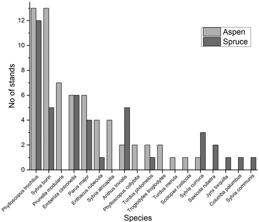
Fig. 2. Number of stands of each stand type (hybrid aspen or spruce regenerations) in which each bird species were encountered.
| Table 4. Generalized linear models (GLM) of species richness in relation to stand type, stand- and landscape variables. For each model the estimated parameters, SE of the parameter estimates as well as t- and p-statistics together with r-square and AIC are presented. See Table 1 for explanation of the variables. Note that the set of variables used in GLM 6 implies multicollinearity, why the individual parameters should be interpreted with care. The overall fit and AIC is, however, comparable with the other GLMs. |
| | | α/β | SE | t | p | R2 | AIC |
| GLM 1 | Intercept | 1.07 | 0.10 | 10.22 | <0.001 | 0.31 | 95.98 |
| | Stand type | 0.52 | 0.15 | 3.51 | 0.002 | | |
| GLM 2 | | | | | | 0.34 | 102.82 |
| GLM 3 | | | | | | 0.54 | 101.58 |
| GLM 4 | | | | | | 0.34 | 104.95 |
| GLM 5 | Intercept | 3.14 | 0.72 | 4.374 | <0.001 | 0.69 | 95.27 |
| | Stand type | –2.86 | 0.90 | –3.182 | 0.007 | | |
| | Devel | 19.82 | 17.54 | 1.13 | 0.277 | | |
| | Agric | –3.51 | 1.78 | –1.969 | 0.069 | | |
| | Wetl | –1.90 | 2.80 | –0.68 | 0.508 | | |
| | Conif | –0.01 | <0.01 | –2.971 | 0.010 | | |
| | Decid | –0.02 | 0.01 | –1.733 | 0.105 | | |
| | Stand type: Devel | –34.18 | 27.27 | –1.253 | 0.231 | | |
| | Stand type: Agric | 2.20 | 2.21 | 0.997 | 0.336 | | |
| | Stand type: Wetl | 1.73 | 5.54 | 0.313 | 0.759 | | |
| | Stand type: Conif | 0.02 | 0.01 | 3.649 | 0.003 | | |
| | Stand type: Decid | 0.05 | 0.02 | 2.614 | 0.020 | | |
| GLM 6 | Intercept | 0.66 | 0.33 | 1.977 | 0.061 | 0.51 | 92.89 |
| | Bas tot | 0.18 | 0.09 | 2.083 | 0.050 | | |
| | Bas asp | 0.04 | 0.17 | 0.25 | 0.805 | | |
| | Height | –0.13 | 0.12 | –1.133 | 0.270 | | |
| | Tree spec | 0.13 | 0.05 | 2.713 | 0.013 | | |
| Table 5. Generalized linear models (GLM) of bird abundance in relation to stand type, stand- and landscape variables. For each model the estimated parameters, SE of the parameter estimates as well as t- and p-statistics together with r-square and AIC. See Table 1 for explanation of the variables. Note that the set of variables used in GLM 6 implies multicollinearity, why the individual parameters should be interpreted with care. The overall fit and AIC is, however, comparable with the other GLMs. |
| | | α/β | SE | t | p | R2 | AIC |
| GLM 1 | Intercept | 1.61 | 0.13 | 12.73 | <0.001 | 0.26 | 133.74 |
| | Stand type | 0.56 | 0.18 | 3.14 | 0.004 | | |
| GLM 2 | Intercept | 1.41 | 0.41 | 3.41 | 0.003 | 0.43 | 134.72 |
| | Stand type | 0.41 | 0.19 | 2.14 | 0.045 | | |
| | Stems | <0.01 | <0.01 | 1.97 | 0.062 | | |
| | Ret tree | –0.01 | 0.02 | –0.49 | 0.628 | | |
| | Thin | –0.22 | 0.22 | –0.99 | 0.332 | | |
| | Tree even | 0.05 | 0.89 | 0.06 | 0.955 | | |
| GLM 3 | Intercept | 2.08 | 0.55 | 3.77 | 0.002 | 0.61 | 132.67 |
| | Stand type | –0.65 | 0.88 | –0.74 | 0.471 | | |
| | Stems | <0.01 | <0.01 | 1.90 | 0.076 | | |
| | Ret tree | –0.06 | 0.02 | –2.47 | 0.025 | | |
| | Thin | 0.63 | 0.35 | 1.78 | 0.094 | | |
| | Tree even | –1.59 | 1.21 | –1.32 | 0.207 | | |
| | Stand type:Stems | <0.01 | <0.01 | –0.15 | 0.881 | | |
| | Stand type:Ret tree | 0.12 | 0.05 | 2.29 | 0.036 | | |
| | Stand type:Thin | –1.23 | 0.45 | –2.70 | 0.016 | | |
| | Stand type:Tree even | 2.05 | 1.89 | 1.08 | 0.294 | | |
| GLM 4 | | | | | | 0.38 | 139.28 |
| GLM 5 | | | | | | 0.56 | 139.74 |
| GLM 6 | Intercept | 0.88 | 0.37 | 2.42 | 0.025 | 0.59 | 123.99 |
| | Bas tot | 0.22 | 0.09 | 2.33 | 0.030 | | |
| | Bas asp | –0.05 | 0.19 | –0.30 | 0.769 | | |
| | Height | 0.03 | 0.13 | 0.22 | 0.827 | | |
| | Tree spec | 0.06 | 0.05 | 1.07 | 0.296 | | |
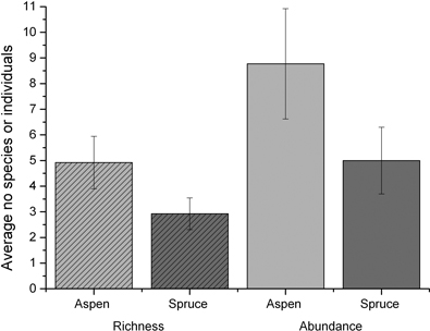
Fig. 3. Average number of bird species (richness) and individuals (abundance) found in hybrid aspen and spruce stands. Error bars show ± two standard errors.
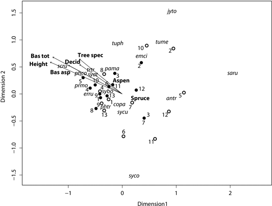
Fig. 4. Ordination diagram from the Non-metric multidimensional scaling showing the two-dimensional final solution with sites (dots) and species. The significant (p ≤ 0.05) environmental variables (names in bold) from a posthoc fit is shown as arrows (continuous) or location in ordination space (factors). Closed dots show the location of aspen sites, while open dots indicate spruce sites. The sites of a spruce/aspen pair have the same number. Phtr is Phylloscopus trochilus, sybo Sylvia borin, prmo Prunella modularis, emci Emberiza citrinella, pama Parus major, erru Erithacus rubecula, syat Sylvia atricapilla, antr Anthus trivialis, phco Phylloscopus collybita, tuph Turdus philomelos, trtr Troglodytes troglodytes, tume Turdus merula, scru Scolopax rusticola, sycu Sylvia curruca, saru Saxicola rubetra, jyto Jynx torquilla, copa Columba palumbus, syco Sylvia communis. A description of the environmental variables can be found in Table 1.
| Table 6. Posthoc fit of environmental variables on the two-dimensional solution from the Non-metric multidimensional scaling. The table shows the independent correlations (continuous) with the two dimensions separately, or location of the centroid (factors) in ordination space together with r-square and p-value for each variable in relation to both dimensions. |
| | NMDS1 corr/centr | NMDS2 corr/centr | r2 | P |
| Bas tot | –0.88 | 0.47 | 0.53 | 0.001 |
| Stems | –0.95 | 0.32 | 0.21 | 0.072 |
| Bas asp | –0.88 | 0.47 | 0.32 | 0.010 |
| Height | –0.91 | 0.40 | 0.53 | 0.002 |
| Ret tree | 0.43 | –0.90 | 0.00 | 0.986 |
| Tree spec | –0.78 | 0.63 | 0.26 | 0.032 |
| Tree even | 0.00 | 1.00 | 0.03 | 0.690 |
| Devel | –0.38 | 0.92 | 0.11 | 0.260 |
| Agric | –0.72 | 0.69 | 0.06 | 0.512 |
| Wetl | –0.86 | –0.51 | 0.09 | 0.339 |
| Conif | 0.80 | –0.61 | 0.16 | 0.134 |
| Decid | –0.82 | 0.57 | 0.23 | 0.043 |
| Spruce stand | 0.21 | –0.13 | 0.15 | 0.013 |
| Aspen stand | –0.21 | 0.13 | | |
| Unthin | –0.09 | 0.00 | 0.05 | 0.315 |
| Thin | 0.24 | –0.00 | | |