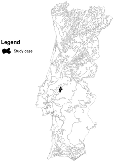
Fig. 1. The map of Portugal and the study area.
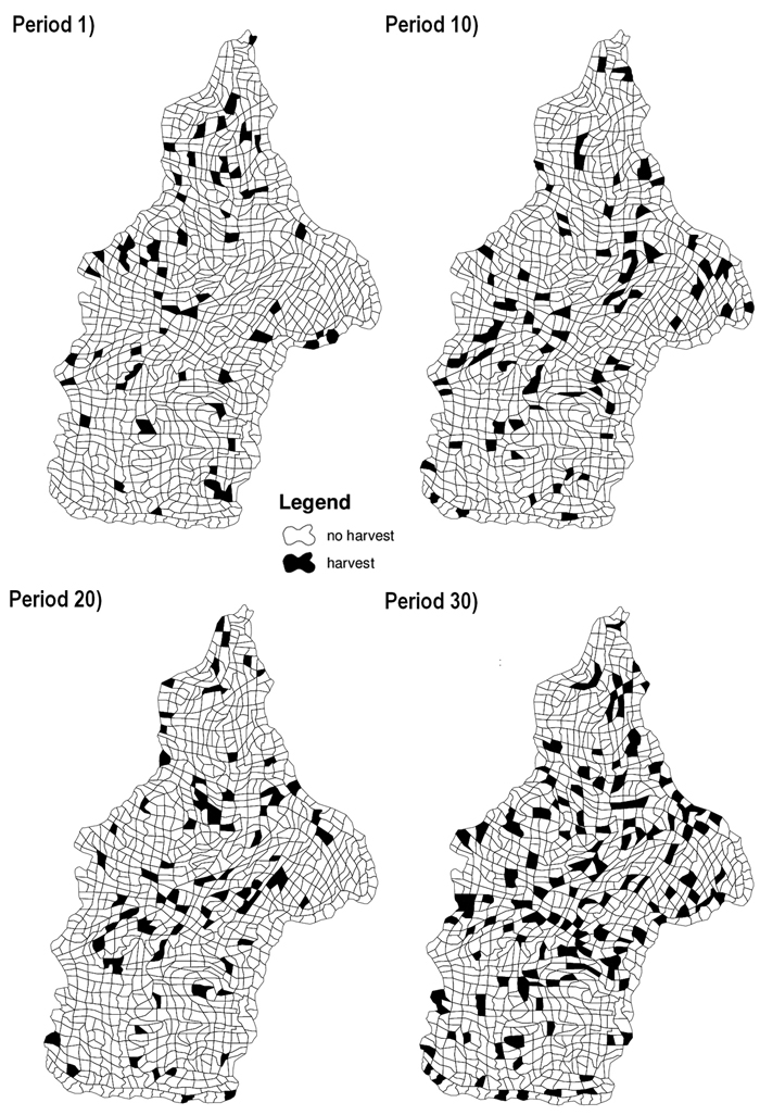
Fig. 2. Maps of study case area presenting harvest schedule generated by Simulated Annealing (SA) for problem III. Stands in black are harvested stands in the corresponding period. Problem III corresponded to the maximization of net returns using even-flow of harvest constraints, ending volume inventory and carbon stock level constraints and adjacency constraints.
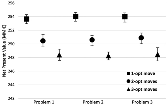
Fig. 3. Performance of the different implementations of Simulated Annealing (SA) (one, two and three-opt moves) for all problem formulations and for the instance of 1000 stands for different combinations of initial temperature (2, 7, 12, 100, 100000) and cooling schedule (0.8, 0.99996). The graph shows the best, the average and the worst solution for each implementation problem. Problem I encompassed the use of even-flow of harvest constraints, Problem II further included the use of ending volume inventory and carbon stock level constraints. Problem III was an extension of previous models and further included adjacency constraints.
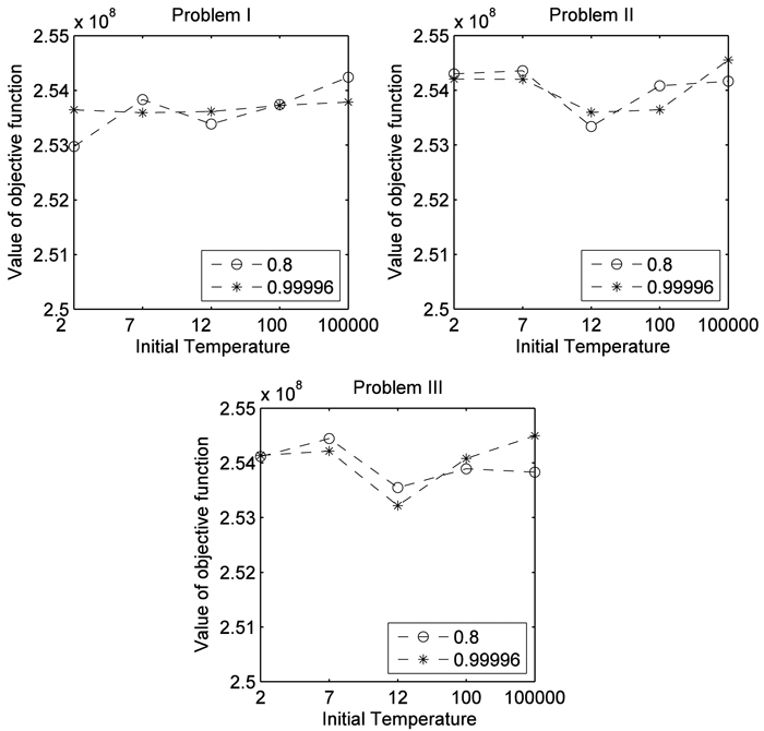
Fig. 4. Comparison of cooling scheduling (0.8 and 0.99996) and initial temperature (2, 7, 12, 100, 100000) for each problem formulation for the instance 1000 stands. Problem I encompassed the use of even-flow of harvest constraints, Problem II further included the use of ending volume inventory and carbon stock level constraints. Problem III was an extension of previous models and further included adjacency constraints.
| Table 1. Configuration of parameters (initial temperature T0, cooling schedule ζ ) for the Instance of 1000 stands. Problem I encompassed the use of even-flow of harvest constraints, Problem II further included the use of ending volume inventory and carbon stock level constraints. Problem III was an extension of previous models and further included adjacency constraints. | |||||||
| Model | Average objective | Best objective | Worst objective | Average time[s] | GAP1 1 [%] | GAP2 2 [%] | Best parameters |
| Problem I | 253654092.6 | 254242073 | 252974250 | 11560 | 0.2313 | 0.499 | T0 = 100000, ζ = 0.8 |
| Problem II | 254044417.2 | 254553811 | 253337282 | 13913 | 0.2 | 0.478 | T0 = 100000, ζ = 0.99996 |
| Problem III | 253998184.9 | 254495562 | 253219220 | 20134 | 0.1954 | 0.502 | T0 = 100000, ζ = 0.99996 |
| 1 GAP1 refers to the relative gap between the best and the average value. | |||||||
| 2 GAP2 refers to the relative gap between the best objective value found and the worst value achieved by SA. | |||||||
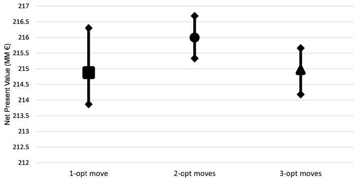
Fig. 5. Performance of the different implementations of Simulated Annealing (SA) (one, two and three-opt moves) for problem formulation III and for the instance of 1000 stands for different combinations of initial temperature and cooling schedule. Problem III corresponded to the maximization of net returns using even-flow of harvest constraints, ending volume inventory and carbon stock level constraints and adjacency constraints.
| Table 2. Comparison of performance of exact (CPLEX) and heuristic (Simulated Annealing (SA)) methods. | ||||||||
| Stands | Problem | CPLEX | SA | Statistics | ||||
| Best objective | Time[s] | Gap[%]3 | Best objective | Average time[s] | Saved time[%] | Relative gap[%]4 | ||
| 100 | I | 19385252 | 6591 | 3.78 | 18208598 | 784 | 88 | 6.07 |
| 100 | II | 18787533 | 24348 | 6.93 | 18247907 | 1039 | 96 | 2.87 |
| 100 | III | 19987548 | 32813 | 0.51 | 18244260 | 1523 | 95 | 8.72 |
| 250 | I | 49576379 | 80 | 0.85 | 47641286 | 2248 | –2710 | 3.90 |
| 250 | II | 49705423 | 148 | 0.58 | 47762817 | 2775 | –1775 | 3.91 |
| 250 | III | 49535258 | 10890 | 0.92 | 47787089 | 4212 | 61 | 3.53 |
| 500 | I | 110140532 | 405 | 0.14 | 107751035 | 4967 | –1126 | 2.17 |
| 500 | II | 109921875 | 523 | 0.33 | 107789228 | 6416 | –1127 | 1.94 |
| 500 | III | 110059776 | 13460 | 0.20 | 107729193 | 9448 | 30 | 2.12 |
| 1000 | I | 261614671 | 8459 | 0.01 | 254242073 | 11560 | –37 | 2.82 |
| 1000 | II | 261604515 | 34076 | 0.01 | 254553811 | 13913 | 59 | 2.70 |
| 1000 | III | - | - | - | 254495562 | 20134 | n.a. | n.a. |
| 3 The column “Gap” refers to the default gap calculation in CPLEX and stands for the relative difference between the highest objective value and the lowest upper bound that is found during optimization process [%]. | ||||||||
| 4 The column “Relative gap” refers to the relative percentage difference between the CPLEX and SA solutions. | ||||||||