| Table 1. Basic characteristics of the forest stands. | ||||
| Month of measurement | GPS | Forest age | Number of trees | Height of tomographic measurement |
| September | 49°18´N, 16°46´E | 100 | 15 | 130 cm |
| October | 49°19´N, 16°45´E | 110 | 12 | 60 cm |
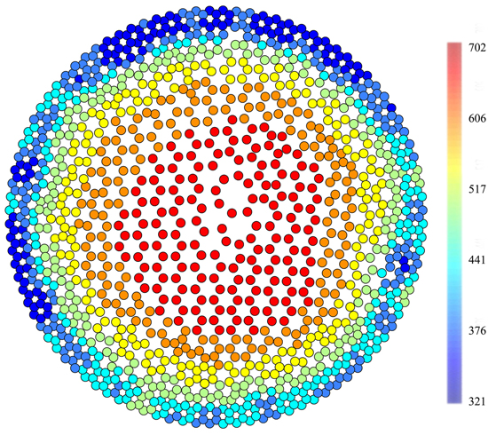
Fig. 1. A tomogram (Ωm) of a healthy individual (September, n. 9) displayed in GIS, when points replace the raster image. There is a clearly visible green transitional boundary between heartwood and sapwood.
| Table 2. Decay quantification and description. While sapwood proportion was found from tomograms, the remaining characteristics, i.e. decay proportion, relative cavity area and decay description, were obtained from radial cuts. | ||||||
| Tree ID | Diameter (cm) | Sapwood propotion (%) | Decay propotion (%) | Relative cavity area (%) | Overall EIT and real cut | Decay description |
| 1 | 123 | 33.7 | - | - | - | - |
| 2 | 122 | 33.1 | - | - | - | - |
| 5 | 169 | 37.5 | - | - | - | - |
| 6 | 132 | 32.3 | - | - | - | - |
| 9 | 153 | 33.3 | - | - | - | - |
| 11 | 147 | 36.0 | - | - | - | - |
| 4B | 137 | 38.1 | - | - | - | - |
| 13 | 146 | 36.7 | - | - | - | - |
| 2B | 218 | 34.1 | 4.8 | - | Fully | 2IR, 1RDS+M |
| 10B | 174 | 31.9 | 6.7 | - | Fully | 3IR |
| 3B | 188 | 42.1 | 7.5 | - | Fully | 1IR, 1RDS+M |
| 12B | 179 | 30.3 | 8.5 | - | Fully | 4IR |
| 8B | 194 | 36.8 | 9.5 | - | Partially | 2VR+M |
| 3 | 131 | 35.4 | 10.5 | - | Partially | 2IR, 1VR |
| 15 | 177 | 36.4 | 11.9 | - | Significantly | 3IR, 1RDS+M |
| 1B | 188 | 43.9 | 13.7 | - | Significantly | 7IR, 2VR |
| 7 | 160 | 41.7 | 17.9 | - | Significantly | 1RDS |
| 7B | 157 | 28.0 | 18.6 | 1.9 | Partially | 1VR, 1RDS+M |
| 11B | 132 | 33.7 | 22.6 | - | Significantly | 4IR, 1VR+M |
| 14 | 140 | 37.5 | 22.8 | - | Significantly | 3IR, 2VR, 1RDS+M |
| 8 | 118 | 38.7 | 32.4 | - | Significantly | 1IR, 1RDS |
| 12 | 178 | 19.2 | 35.2 | - | Partially | 4VR+M, 3RDS+M |
| 6B | 220 | 23.1 | 43 | 6.3 | Significantly | 2VR, 1RDS+M |
| 5B | 173 | 24.8 | 46.4 | 2.1 | Fully | 3RDS+M |
| 10 | 173 | 19.8 | 47 | - | Significantly | 1RDS+M |
| 4 | 128 | 20.4 | 74.4 | - | Significantly | 1RDS |
| 9B | 180 | 19.3 | 85.4 | unknown | Significantly | 1RDS |
| nIR = Incipient rot (early stages) nVR = Visible rot (without destroying the wood structure) nRDS = Advanced rot destroying the wood structure n = The number of occurrences (spots) of rot +M = Mycelium | ||||||
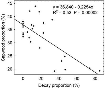
Fig. 2. Relation between a sapwood proportion found through tomography measurements and a decay proportion identified on the radial cut implemented on the site of tomography measurements.
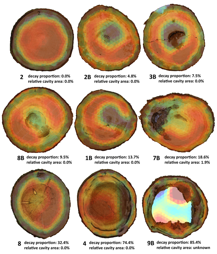
Fig. 3. Cuts with overlapping tomograms being sorted as per decay proportion in the real cut. Present are also three exceptions (1B, 3B, 7B) as described in Section 3.3. Due to the cavity filling deliberately falling out during the felling, the cavity presence and extent could not be determined during the tomography measurement.
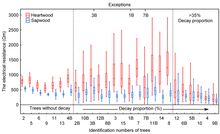
Fig. 4. Electrical resistance values split into heartwood and sapwood data. Sorted by decay proportion (as measured on radial cuts). The central rectangle spans the first quartile (Q1-25%) to the third quartile (Q3-75%). A segment inside the rectangle shows the median and “whiskers” above and below the box show the locations of the minimum and maximum (1%).