| Table 1. Derivation of mean volume growth sub-model. | |||
| Model | Invariant | Differential equation | Transition function |
| E1 | 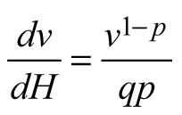 | 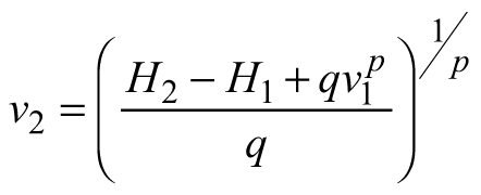 | |
| E2 | 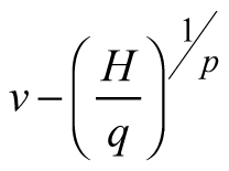 | 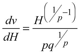 | 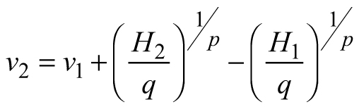 |
| E3 | 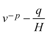 | 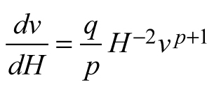 | 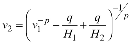 |
| Abbreviations: v − mean stem volume (m3) and H − dominant stand height (m); p, q – global model parameters | |||
| Table 2. Description of the data set. | ||||
| Stand variable | Mean | Standard deviation | Minimum | Maximum |
| DBH (cm) | 17.7 | 6.0 | 5.6 | 34.7 |
| N (trees ha–1) | 2270 | 1862 | 393 | 9305 |
| H (m) | 16.3 | 5.0 | 6.3 | 32.5 |
| Age (years) | 38 | 14 | 12 | 80 |
| v (m3) | 0.260 | 0.218 | 0.011 | 1.257 |
| y (m3 ha–1) | 340.7 | 144.6 | 61.4 | 723.4 |
| Abbreviations: DBH – diameter at breast height; H − dominant stand height; N – stand density; v – mean stem volume; y – total stand volume | ||||
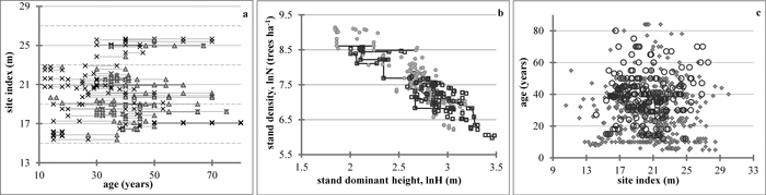
Fig. 1. Data examination charts. a – Stand age-site index data range of this study. Basal area values below (×) and above (▲) average are indicated. Solid lines connect measurements of the same plot, for site index averaged per plot. Dotted gridlines delimit 4m-site index classes. b – Dominant stand height-stand density data range. Site index values below (●) and above (□) average are indicated. Thinning trajectories for some of the managed plots are represented by solid lines; c – Site index-stand age data comparison between the permanent sample plots of this study (◌) and temporary sample plot data (♦). Site index model by Stankova and Diéguez-Aranda (2012) for reference age 50 years and temporary sample plots data from Stankova and Shibuya (2007) are used. View larger in new window/tab.
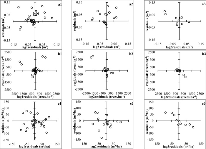
Fig. 2. Plots of residuals vs lag−residuals. a1 to a3 – mean stem volume, m3; b1 to b3 – stand density, ha-1; c1 to c3 – total stand volume m3/ha. View larger in new window/tab.
| Table 3. Goodness - of - fit statistics for the whole-stand dynamic model. | |||||||
| Global model parameters | Regression estimation a | ||||||
| Parameter: Estimate | p: 0.4740 | Dependent variable | Adj. R2 | RMSE | Bias b | Relative bias (%) b | |
| ASE HCCME | 0.0207 0.0556 | ||||||
| Parameter: Estimate | q: 37.934 | Stand density | 0.948 | 403 | –11 | –0.37 | |
| ASE HCCME | 2.9410 9.1053 | ||||||
| Mean stem volume (projected) | 0.931 | 0.0460 | –0.0002 | –2.42 | |||
| Parameter: Estimate | r: –0.0945 | ||||||
| ASE HCCME | 0.0067 0.0402 | Mean stem volume (predicted) | 0.740 | 0.0893 | 0.0034 | –10.68 | |
| Parameter: Estimate | s: 69.279 | ||||||
| ASE HCCME | 8.6749 27.317 | Total stand volume | 0.919 | 41.81 | –0.480 | –1.89 | |
| Abbreviations: ASE – Asymptotic Standard Error; HCCME – Heteroscedasticity - Consistent Covariance Matrix Estimator; Adj. R2 – adjusted coefficient of determination; RMSE – Root Mean Square Error. a Total number of observations N = 239. b The absolute and relative biases for all estimated stand variables are not significantly different from zero. | |||||||
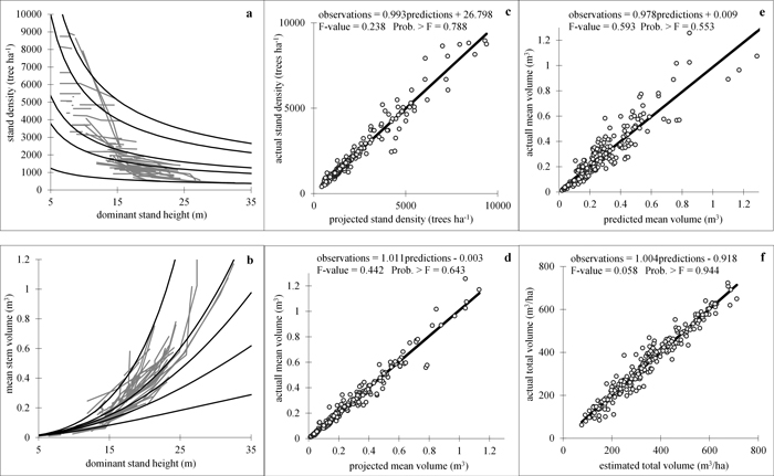
Fig. 3. Goodness-of-fit and prediction charts. a, b − density decrease (a) and volume growth (b) models fitted to the experimental data. Fitted curves for five data series comprising the data range are shown; c, d actual vs. projected values: stand density (c) and mean stem volume (d); e − actual vs. predicted mean stem volume; f − actual vs. estimated total stand volume. Linear regressions of observed against estimated variable values are fitted and the results from simultaneous F-test for line slope equals 1 and zero intercept (Gadow and Hui 1999) are shown in the plots. View larger in new window/tab.
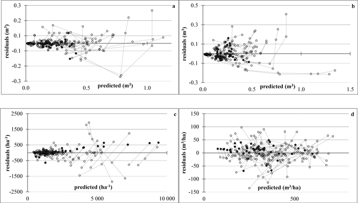
Fig. 4. Plots of residuals vs. predicted values. a – projected mean stem volume; b – predicted mean stem volume; c – stand density; d – total stand volume. The lines connect the residuals (◌) by data series, the symbol ● denoting values of just-thinned plots. View larger in new window/tab.
| Table 4. Validation test statistics of the whole-stand dynamic model. | ||||||
| Dependent variable | Tolerance intervals (TI) for the relative errors 1 – α = 99% probability for the future errors | |||||
| 1 – γ = 50% | 1 – γ = 75% | 1 – γ = 95% | ||||
| of future observations | ||||||
| Stand density | –19.6 | 17.6 | –32.7 | 30.7 | –54.9 | 53.0 |
| Projected mean stem volume | –17.4 | 16.4 | –29.4 | 28.4 | –49.7 | 48.7 |
| Predicted mean stem volume | –33.4 | 12.9 | –49.8 | 29.2 | –77.5 | 57.0 |
| Total stand volume | –18.8 | 19.2 | –32.2 | 32.6 | –54.9 | 55.4 |