| Table 1. Mire types of the pristine, drained and restored treatments prior to the start of restoration in 2003, in the nine study mires in Central Finland and Northern Karelia, and their approximate coordinates. N = number of sampling locations representing the given mire type (total = 162 sampling locations). | |||
| Region/mire | Treatment | Mire types1 (N) | Coordinates |
| Central Finland | |||
| Kiemanneva | Pristine | IR (1), RiNR (3), TR (2) | 63°23´N, 25°16´E |
| Drained | muIR (3), TKg (3) | ||
| Restored | muIR (3), muRaR(3) | ||
| Väljänneva | Pristine | LkN (2), RaR(1), SR (3) | 63°19´N, 25°18´E |
| Drained | muIR (1), muRaR (3), muTR (1), TKg (1) | ||
| Restored | muIR (1), muKeR (3), muRaR (2) | ||
| Southern Kulhanvuori | Pristine | IR (1), SR (1), TR (4) | 62°34´N, 24°57´E |
| Drained | muIR (1), TKg (5) | ||
| Restored | muIR (3), TKg (3) | ||
| Northern Kulhanvuori | Pristine | LkR (6) | 62°35´N, 24°57´E |
| Drained | muRaR (1), TKg (5) | ||
| Restored | muRaR (1), TKg (5) | ||
| Northern Karelia | |||
| Ristisuo | Pristine | LkR (1), RaR (5) | 62°56´N, 31°20´E |
| Drained | muIR (3), muKgR (1), muRaR (2) | ||
| Restored | muIR (4), muPsR (1), muRaR (1) | ||
| Juurikkasuo | Pristine | LkR (1), RaR (5) | 62°56´N, 31°26´E |
| Drained | muIR (2), muKgR (1), TKg (2), VT (1) | ||
| Restored | muPsR (1), TKg (5) | ||
| Rapalahdensuo | Pristine | LkR (4), RaR (2) | 62°54´N, 29°30´E |
| Drained | muIR (2), muLkR (1), muRaR (1), TKg (2) | ||
| Restored | muIR (4), TKg (2) | ||
| Tiaissuo | Pristine | LkR (3), RaR (3) | 62°56´N, 29°24´E |
| Drained | muIR (4), TKg (2) | ||
| Restored | muIR (4), muRaR (2) | ||
| Heinäsuo | Pristine | LkN (1), RaR (5) | 62°54´N, 31°28´E |
| Restored-a | muIR (3), muLkR (2), muRaR (1) | ||
| Restored-b | LkR (1), muIR (4), muLkR (1) | ||
| 1 Mire type abbreviations are according to Eurola et al. (1995), and English translations are according to Raunio et al. (2008): IR = Dwarf shrub pine bogs, LkN = Low-sedge bogs & fens, LkR = Low-sedge pine fens, muIR = Transforming Dwarf shrub pine bogs, muKeR = Transforming Ridge-hollow pine bogs, muKgR = Transforming Thin-peated pine mires, muLkR = Transforming Low-sedge pine fens, muPsR = Transforming Carex globularis pine mires, muRaR = Transforming Sphagnum fuscum bogs, muTR = Transforming Eriophorum vaginatum pine bogs, RiNR = Flark pine fens, RaR = Sphagnum fuscum bogs, SR = Tall-sedge pine fens, TKg = Transformed drained mires, TR = Eriophorum vaginatum pine bogs, VT = Sub-xeric heath forests. | |||
| Table 2. Mean ( | ||||||||||||
| Variable | Treatment | Test statistics | ||||||||||
| Pristine (N = 54) | Drained (N = 48) | Restored (N = 60) | ||||||||||
| SE | SE | SE | H | p adj. | ||||||||
| Living trees (h > 1.5 m): | ||||||||||||
| Total number of stems | 5.8 | 1.0 | a | 23.1 | 2.5 | b | 9.2 | 1.2 | a | 60.47 | <0.0001 | |
| No. of pines | 5.8 | 1.0 | a | 14.9 | 1.3 | b | 8.0 | 1.2 | a | 42.03 | <0.0001 | |
| No. of birches | 0.1 | 0.0 | a | 7.4 | 2.3 | b | 1.2 | 0.4 | a | 42.95 | <0.0001 | |
| No. of stems d1.3 < 7 cm | 4.7 | 0.8 | a | 13.8 | 2.3 | b | 7.1 | 1.1 | a | 17.65 | 0.0007 | |
| No. of stems d1.3 7–20 cm | 1.0 | 0.3 | a | 8.2 | 0.8 | b | 1.8 | 0.3 | a | 67.34 | <0.0001 | |
| No. of stems d1.3 > 20 cm | 0.0 | 0.0 | a | 1.1 | 0.2 | b | 0.3 | 0.1 | a | 32.44 | <0.0001 | |
| No. of stems h 1.5–3 m | 4.1 | 0.7 | 3.5 | 0.8 | 3.5 | 0.8 | 2.05 | 1.0000 | ||||
| No. of stems h 3–8 m | 1.7 | 0.3 | a | 12.5 | 2.0 | b | 4.9 | 0.7 | c | 40.24 | <0.0001 | |
| No. of stems h > 8 m | 0.0 | 0.0 | a | 7.0 | 1.2 | b | 0.8 | 0.4 | a | 68.29 | <0.0001 | |
| Number of species | 0.9 | 0.1 | a | 1.8 | 0.1 | b | 1.0 | 0.1 | a | 53.10 | <0.0001 | |
| Dead trees: | ||||||||||||
| Total number of snags | 0.7 | 0.2 | 1.1 | 0.2 | 0.9 | 0.3 | 1.49 | 1.0000 | ||||
| No. of snags d1.3 < 7 cm | 0.6 | 0.1 | 0.9 | 0.2 | 0.8 | 0.3 | 0.96 | 1.0000 | ||||
| No. of snags d1.3 7–20 cm | 0.1 | 0.1 | 0.2 | 0.1 | 0.1 | 0.0 | 1.16 | 1.0000 | ||||
| Total number of logs | 0.0 | 0.0 | a | 0.4 | 0.2 | a | 0.6 | 0.2 | a | 10.24 | 0.0354 | |
| No. of logs d1.3 < 7 cm | 0.0 | 0.0 | a | 0.4 | 0.2 | a | 0.6 | 0.2 | a | 11.15 | 0.0235 | |
| No. of logs d1.3 7–20 cm | 0.0 | 0.0 | 0.1 | 0.0 | 0.1 | 0.0 | 1.57 | 1.0000 | ||||
| No. of logs d1.3 > 20 cm | 0.0 | 0.0 | 0.0 | 0.0 | 0.0 | 0.0 | 1.70 | 1.0000 | ||||
| Tree saplings (h 50–150 cm): | ||||||||||||
| Total number of saplings | 1.9 | 0.3 | 2.6 | 0.6 | 1.7 | 0.3 | 1.02 | 1.0000 | ||||
| No. of pines | 1.9 | 0.3 | a | 1.4 | 0.4 | b | 1.2 | 0.2 | ab | 8.60 | 0.0736 | |
| No. of birches | 0.0 | 0.0 | a | 0.9 | 0.4 | b | 0.3 | 0.1 | ab | 17.14 | 0.0014 | |
| Number of species | 0.7 | 0.1 | 0.9 | 0.1 | 0.8 | 0.1 | 1.31 | 1.0000 | ||||
| Microsite types (%): | ||||||||||||
| Hummock | 46.1 | 3.6 | a | 96.6 | 2.0 | b | 66.9 | 4.1 | c | 71.47 | <0.0001 | |
| Lawn | 37.8 | 4.0 | a | 1.1 | 0.7 | b | 24.8 | 3.8 | c | 58.68 | <0.0001 | |
| Flark | 15.5 | 3.6 | a | 0.0 | 0.0 | b | 6.3 | 1.7 | a | 27.05 | <0.0001 | |
| Mire-surface coverage (%): | ||||||||||||
| Water | 0.0 | 0.0 | a | 0.0 | 0.0 | a | 2.4 | 1.0 | a | 14.20 | 0.0052 | |
| Litter | 2.4 | 1.2 | a | 12.1 | 3.1 | ab | 15.5 | 2.4 | b | 27.30 | <0.0001 | |
| Sphagnum spp. | 90.0 | 1.7 | a | 30.7 | 3.8 | b | 46.0 | 3.9 | b | 83.39 | <0.0001 | |
| Other mosses | 3.1 | 0.6 | a | 38.4 | 3.9 | b | 22.7 | 2.8 | c | 64.53 | <0.0001 | |
| Herbs, sedges and grasses | 14.0 | 1.1 | a | 8.2 | 1.0 | b | 20.9 | 2.2 | a | 22.51 | <0.0001 | |
| Low dwarf shrubs | 9.6 | 1.2 | ab | 16.6 | 2.1 | a | 8.6 | 1.3 | b | 8.92 | 0.0655 | |
| Tall dwarf shrubs | 3.7 | 0.6 | a | 6.2 | 0.8 | ab | 9.5 | 1.0 | b | 19.39 | 0.0007 | |
| Water-table depth (cm below the mire-surface) | 15.1 | 1.3 | a | 38.0 | 1.5 | b | 16.0 | 1.3 | a | 74.34 | <0.0001 | |
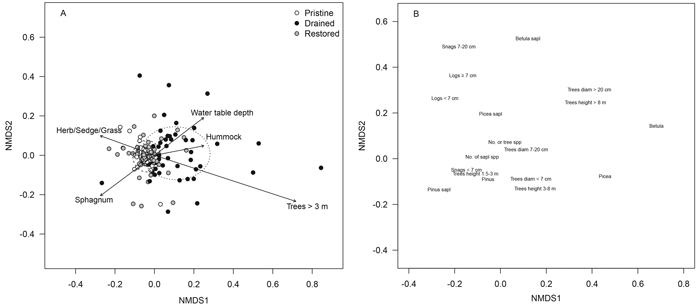
Fig. 1. NMDS ordination plots of the tree-stand variables presenting (A) sampling locations of the pristine (white dots), drained (black dots) and restored (grey dots) mires and (B) tree and sapling variables within the sampling locations. The dispersion ellipses in plot A indicate 1 SD of the weighted average of the site scores of pristine (solid line), drained (dotted line) and restored (dashed line) mires. The arrows in plot A indicate the environmental variables fitted to the ordination space such that only variables with highly significant p-values are shown (p < 0.001; the direction of the arrow indicates the direction of the gradient, and the length of the arrow indicates the strength of the correlation). View larger in new window/tab.
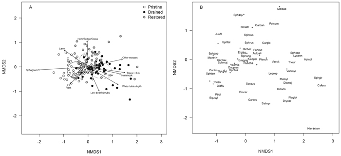
Fig. 2. NMDS ordination plots of the floristic data presenting (A) sampling locations of the pristine (white dots), drained (black dots) and restored (grey dots) mires and (B) moss, lichen and vascular plant species within the sampling locations (note the differences in the scales of axes between plots A and B). The dispersion ellipses in plot A indicate 1 SD of the weighted average of the site scores of pristine (solid line), drained (dotted line) and restored (dashed line) mires. The arrows in plot A indicate the environmental variables fitted to the ordination space such that only variables with highly significant p-values are shown (p < 0.001). The species names indicated in plot B are such that for overlapping labels, priority is given to the most abundant species and the rest are indicated with “+”. After this, 14 frequent species (occurring in > 9% of sampling locations) remained without labels. These species are located as follows: Dicranum polysetum ca. 0.7 units right from the origin, Vaccinium uliginosum, Chamaedaphne calyculata, Polytrichum strictum Menzies ex Brid., Vaccinium oxycoccos, Betula nana, Sphagnum magellanicum Brid. and Andromeda polifolia within ca. 0.3 units from the origin, Carex rostrata Stokes ca. 1.0 units left from the origin, Pinus sylvestris L., Calluna vulgaris, Mylia anomala (Hook.) Gray, Drosera rotundifolia and Sphagnum rubellum within ca. 0.5–1.0 units toward the ca. lower left corner from the origin. For species abbreviations, see Appendix 1 (abbreviations represent the first three letters of the genus name and the first three letters of the species name). View larger in new window/tab.
| Table 3. Mean ( | ||||||||||||||||||||||||||
| Species | Mire type1 | Test statistics | ||||||||||||||||||||||||
| Pristine | Transforming and transformed | |||||||||||||||||||||||||
| LkR (N = 15) | RaR (N = 21) | SR (N = 4) | TR (N = 6) | muRaR (N = 7) | muIR (N = 16) | TKg (N = 20) | ||||||||||||||||||||
| fr | fr | fr | fr | fr | fr | fr | G2 | p adj. | ||||||||||||||||||
| Ant workers | ||||||||||||||||||||||||||
| Formica picea | 0.5 | 7 | 0.3 | 7 | 0.8 | 3 | 0.3 | 2 | 0.0 | 0 | 0.0 | 0 | 0.1 | 1 | 27.30 | 0.0010 | ||||||||||
| Formica uralensis | 0.1 | 2 | 0.0 | 0 | 0.0 | 0 | 0.2 | 1 | 0.3 | 2 | 0.2 | 3 | 0.2 | 3 | 8.66 | 0.7269 | ||||||||||
| Myrmica scabrinodis | 0.6 | 9 | 0.9 | 18 | 0.8 | 3 | 0.7 | 4 | 0.9 | 6 | 0.6 | 10 | 0.4 | 7 | 13.90 | 0.1592 | ||||||||||
| Lasius platythorax | 0.3 | 4 | 0.4 | 9 | 0.5 | 2 | 0.5 | 3 | 0.3 | 2 | 0.5 | 8 | 0.5 | 10 | 3.25 | 1.0000 | ||||||||||
| Formica sanguinea | 0.1 | 2 | 0.4 | 9 | 0.3 | 1 | 0.0 | 0 | 0.4 | 3 | 0.1 | 1 | 0.1 | 1 | 16.86 | 0.0579 | ||||||||||
| Leptothorax acervorum | 0.2 | 3 | 0.4 | 9 | 0.5 | 2 | 0.2 | 1 | 0.1 | 1 | 0.1 | 1 | 0.1 | 2 | 11.43 | 0.3491 | ||||||||||
| Myrmica rubra | 0.1 | 2 | 0.1 | 2 | 0.3 | 1 | 0.0 | 0 | 0.0 | 0 | 0.1 | 1 | 0.2 | 3 | 4.43 | 1.0000 | ||||||||||
| Myrmica ruginodis | 0.3 | 5 | 0.4 | 9 | 0.0 | 0 | 0.3 | 2 | 0.9 | 6 | 0.9 | 15 | 0.9 | 18 | 36.74 | < 0.0001 | ||||||||||
| Camponotus herculeanus | 0.1 | 1 | 0.0 | 0 | 0.0 | 0 | 0.2 | 1 | 0.1 | 1 | 0.8 | 12 | 0.7 | 14 | 51.34 | < 0.0001 | ||||||||||
| Ant queens | ||||||||||||||||||||||||||
| Myrmica scabrinodis | 0.2 | 3 | 0.3 | 7 | 1.0 | 4 | 0.5 | 3 | 0.1 | 1 | 0.3 | 4 | 0.0 | 0 | 25.74 | 0.0017 | ||||||||||
| Myrmica ruginodis | 0.1 | 2 | 0.0 | 0 | 0.0 | 0 | 0.0 | 0 | 0.3 | 2 | 0.6 | 9 | 0.5 | 9 | 29.93 | < 0.0001 | ||||||||||
| Mean number of species | H | p adj. | ||||||||||||||||||||||||
| Mire ants | 1.3 | 0.2 | 1.2 | 0.1 | 1.8 | 0.3 | 1.3 | 0.4 | 1.1 | 0.1 | 0.9 | 0.2 | 0.6 | 0.1 | 20.45 | 0.0158 | ||||||||||
| All ants | 2.4 | 0.3 | 3.0 | 0.3 | 3.3 | 0.5 | 2.5 | 0.8 | 3.3 | 0.4 | 3.5 | 0.3 | 3.6 | 0.3 | 8.82 | 0.7269 | ||||||||||
| 1Mire type abbreviations are according to Eurola et al. (1995), and English translations are according to Raunio et al. (2008): LkR = Low-sedge pine fens, RaR = Sphagnum fuscum bogs, SR = Tall-sedge pine fens, TR = Eriophorum vaginatum pine bogs, muRaR = Transforming Sphagnum fuscum bogs, muIR = Transforming Dwarf shrub pine bogs, TKg = Transformed drained mires. | ||||||||||||||||||||||||||
| Table 4. Mean ( | |||||||||||
| Species | Treatment | Test statistics | |||||||||
| Pristine (N = 54) | Drained (N = 48) | Restored (N = 60) | |||||||||
| fr | fr | fr | G2 | p adj. | |||||||
| Ant workers: | |||||||||||
| Formica picea | 0.44 | 24 | 0.02 | 1 | 0.02 | 1 | 48.63 | < 0.0001 | |||
| Formica uralensis | 0.07 | 4 | 0.19 | 9 | 0.08 | 5 | 3.76 | 0.6328 | |||
| Myrmica scabrinodis | 0.74 | 40 | 0.52 | 25 | 0.67 | 40 | 5.49 | 0.2918 | |||
| Lasius platythorax | 0.35 | 19 | 0.50 | 24 | 0.60 | 36 | 7.13 | 0.1431 | |||
| Formica sanguinea | 0.22 | 12 | 0.13 | 6 | 0.23 | 14 | 2.44 | 1.0000 | |||
| Leptothorax acervorum | 0.30 | 16 | 0.15 | 7 | 0.20 | 12 | 3.52 | 0.6513 | |||
| Myrmica rubra | 0.09 | 5 | 0.13 | 6 | 0.10 | 6 | 0.30 | 1.0000 | |||
| Myrmica ruginodis | 0.37 | 20 | 0.92 | 44 | 0.72 | 43 | 37.34 | < 0.0001 | |||
| Camponotus herculeanus | 0.06 | 3 | 0.67 | 32 | 0.30 | 18 | 47.23 | < 0.0001 | |||
| Ant queens: | |||||||||||
| Myrmica scabrinodis | 0.41 | 22 | 0.10 | 5 | 0.18 | 11 | 14.25 | 0.0061 | |||
| Myrmica ruginodis | 0.04 | 2 | 0.42 | 20 | 0.28 | 17 | 24.99 | < 0.0001 | |||
| Camponotus herculeanus | 0.11 | 6 | 0.02 | 1 | 0.20 | 12 | 9.68 | 0.0450 | |||
| Mean number of species: | H | p adj. | |||||||||
| Mire ants | 1.3 | 0.1 | a | 0.8 | 0.1 | b | 0.8 | 0.1 | b | 22.59 | < 0.0001 |
| All ants | 2.7 | 0.2 | a | 3.6 | 0.2 | b | 3.1 | 0.1 | ab | 10.23 | 0.0390 |
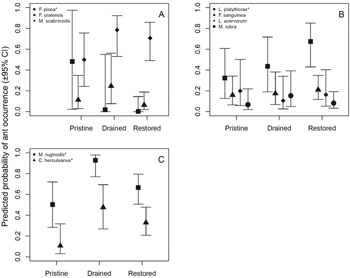
Fig. 3. Statistical responses of individual ant species to mire treatment (A = mire specialist species, B = generalist species, C = forest species). * = statistically significant (p < 0.05) responses (see Table 5).
| Table 5. Generalised linear mixed model results of ant mire specialists, generalists and forest species. Model estimates, standard errors (SE) and p-values of terms retained in the models are given. Treatment, Sphagnum cover, hummock cover and number of trees (> 3 m) were a priori chosen as important environmental variables for the ant occurrences and were retained in all final models. Other variables were subject to model selection and their values are only given when they remained in the final model. Statistically significant p-values (< 0.05) are in bold. The intercept represents prediction in the pristine mire treatment. Est. = Estimate. * = mire specialist species, ** = generalist species, *** = forest species, all according to our a priori evaluations. View in new window/tab. |
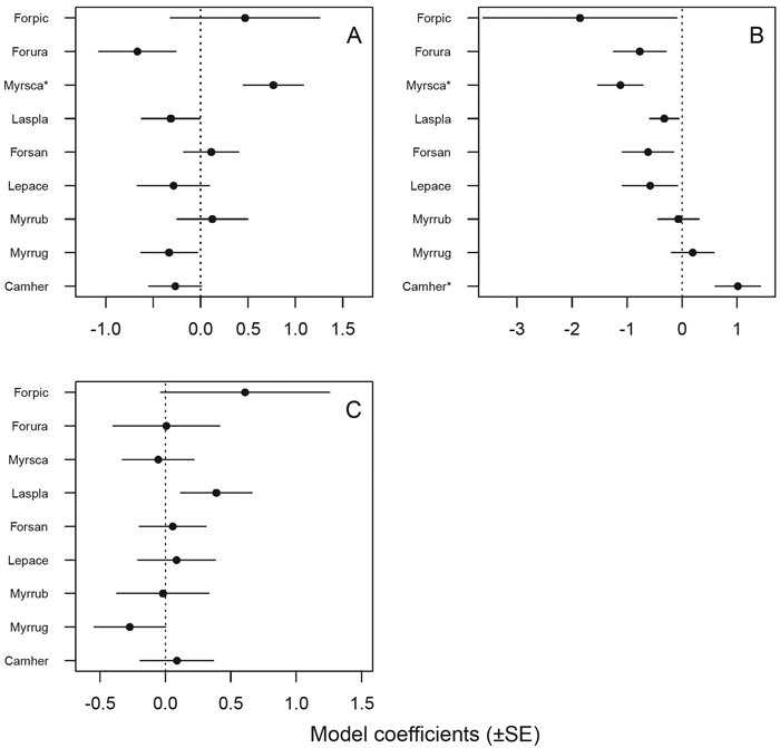
Fig. 4. Statistical responses (model coefficients ± SE, see Table 5) of individual ant species to environmental variables: A = Sphagnum moss cover, B = number of tall trees (> 3 m), C = hummock cover. * = statistically significant (p < 0.05) responses. Species were listed a priori (based on expert opinion and the literature: Krogerus 1960; Vepsäläinen et al. 2000; Punttila and Kilpeläinen 2009) from the most mire-associated (mire specialist) species at the top of each plot to species with the strongest forest affinities (forest species) at the bottom of each plot; generalist species are located in-between.
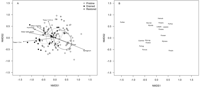
Fig. 5. NMDS ordination plots of the ant data presenting (A) sampling locations of the pristine (white dots), drained (black dots) and restored (grey dots) mires and (B) ant species within the sampling locations. The dispersion ellipses in plot A indicate 1 SD of the weighted average of the site scores of pristine (solid line), drained (dotted line) and restored (dashed line) mires. The arrows in plot A indicate the environmental variables fitted to the ordination space such that only variables with highly significant p-values are shown (p < 0.001). For species abbreviations, see Appendix 2 (abbreviations represent the first three letters of the genus name and the first three letters of the species name). View larger in new window/tab.