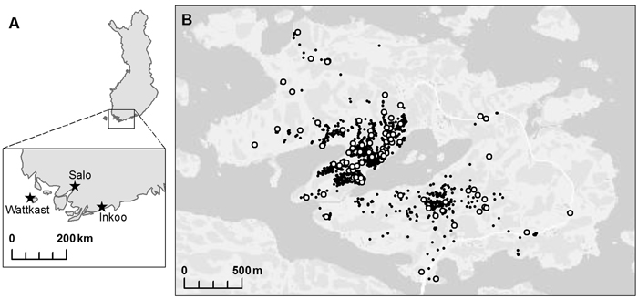
Fig. 1. A map of the populations of Quercus robur investigated at (A) the regional and (B) the landscape level. Within the island of Wattkast (B), each individual oak tree is indicated with a small black dot (N = 1900) and the trees sampled for the genetic analysis (n = 194) with large white dots.
| Table 1. Genetic variation (number of alleles (Â35 or A), expected heterozygosity (He), and observed heterozygosity (Ho)) at 15 microsatellite loci in the populations of Wattkast, Inkoo and Salo. For the Salo population, data is missing for locus ssrQrZAG 108. For the Wattkast and Inkoo populations, Â35 refers to the expected number of alleles after rarefaction to a random sample of 35 individuals. | |||||||||
| Wattkast | Inkoo | Salo | |||||||
| Locus | Â35 | He | Ho | Â35 | He | Ho | A | He | Ho |
| ssrQpZAG1101 | 8.53 | 0.71 | 0.50 | 13.18 | 0.66 | 0.66 | 11 | 0.70 | 0.79 |
| ssrQpZAG151 | 6.08 | 0.68 | 0.60 | 8.38 | 0.52 | 0.53 | 3 | 0.25 | 0.09 |
| ssrQpZAG1/51 | 7.38 | 0.72 | 0.57 | 10.44 | 0.88 | 0.95 | 11 | 0.88 | 0.85 |
| ssrQpZAG161 | 11.64 | 0.78 | 0.72 | 15.56 | 0.91 | 0.89 | 13 | 0.86 | 1.00 |
| ssrQpZAG361 | 9.66 | 0.81 | 0.64 | 10.30 | 0.85 | 0.82 | 9 | 0.83 | 0.97 |
| ssrQpZAG91 | 9.39 | 0.81 | 0.75 | 9.95 | 0.87 | 0.77 | 11 | 0.73 | 0.74 |
| ssrQpZAG1041 | 11.43 | 0.83 | 0.80 | 18.92 | 0.90 | 0.88 | 14 | 0.90 | 0.90 |
| MSQ132 | 5.45 | 0.27 | 0.25 | 9.03 | 0.70 | 0.67 | 5 | 0.70 | 0.58 |
| MSQ42 | 8.07 | 0.74 | 0.31 | 7.76 | 0.83 | 0.62 | 5 | 0.75 | 0.72 |
| ssrQrZAG 1013 | 7.60 | 0.71 | 0.60 | 15.71 | 0.88 | 0.85 | 11 | 0.81 | 0.78 |
| ssrQrZAG 1083 | 8.51 | 0.70 | 0.65 | 13.34 | 0.74 | 0.60 | - | - | - |
| ssrQrZAG 113 | 13.34 | 0.88 | 0.75 | 20.88 | 0.91 | 0.88 | 15 | 0.90 | 0.91 |
| ssrQrZAG 1123 | 8.29 | 0.70 | 0.68 | 16.09 | 0.91 | 0.97 | 11 | 0.84 | 0.91 |
| ssrQrZAG 73 | 11.16 | 0.85 | 0.80 | 15.73 | 0.90 | 0.90 | 10 | 0.86 | 0.91 |
| ssrQrZAG 873 | 13.89 | 0.86 | 0.87 | 16.32 | 0.90 | 0.89 | 13 | 0.86 | 1.00 |
| Mean | 9.37 | 0.74 | 0.63 | 13.44 | 0.82 | 0.79 | 10.14 | 0.72 | 0.80 |
| s.d. | 2.50 | 0.15 | 0.17 | 4.00 | 0.12 | 0.14 | 3.55 | 0.26 | 0.24 |
| 1 Reference: Steinkellner et al. 1997. 2 Reference: Dow et al. 1995. 3 Reference: Kampfer et al. 1998. | |||||||||
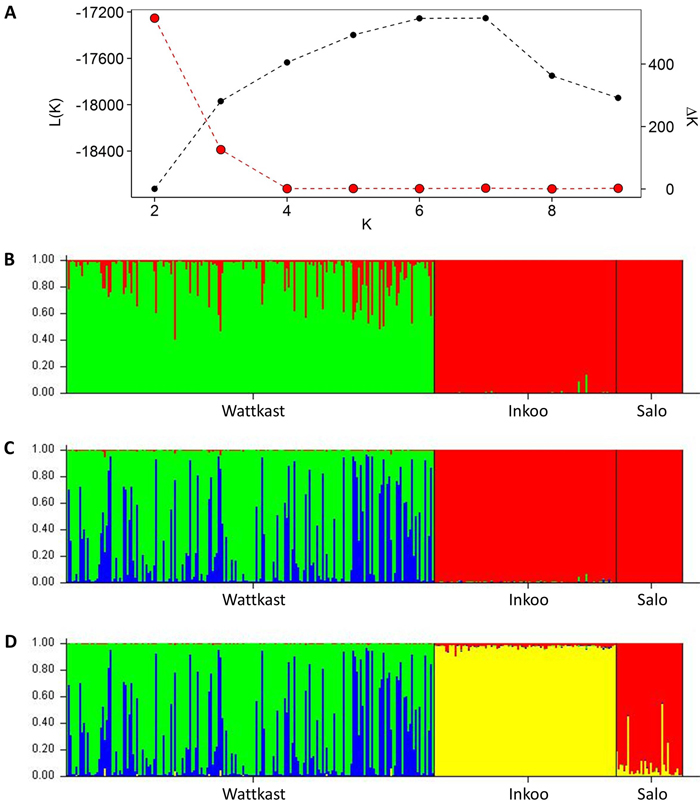
Fig. 2. Inference of genetic clusters within the populations of study based on the population assignment analysis implemented using the software STRUCTURE. Shown are the log-likelihood values of the data given a number of clusters (K) assumed (L(K); black dots in panel A) and the rate of change of L(K) (∆K; red dots in panel A). Bar plots in panels B–D show the results of the simulation for given value of K; (B) K = 2; (C) K = 3; (D) K = 4. Here, each vertical bar represents an individual, the different colors represent the genetic groups identified by the analysis, and the coloration of each bar indicates the probability with which an individual can be assigned to a particular ancestry. The three populations sampled are separated by black vertical lines.
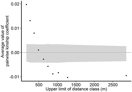
Fig. 3. Associations between genetic relatedness and geographic distance among pairs of individual trees on Wattkast. Black dots show average values of observed pairwise kinship coefficients within 10 distance classes, and grey area shows 95% confidence interval of values derived from permutations of individual locations among all individuals.
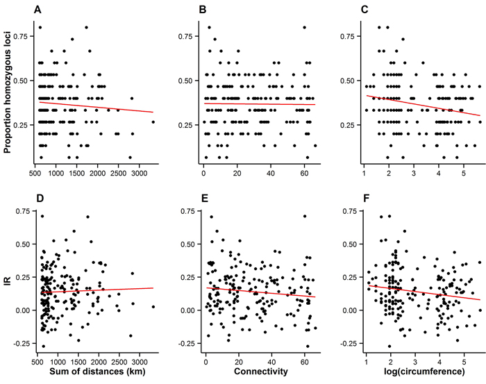
Fig. 4. Measures of individual inbreeding (proportion homozygous loci, A–C, and internal relatedness (IR), D–E) plotted against the connectivity (A–B and D–E), and the size of trees on Wattkast (natural logarithm of circumference; C and F). Red lines represent lines of best fit. Statistically significant associations were found between the proportion of homozygous loci and tree size (C; slope = −0.02 ± 0.008, P = 0.002) and between IR and tree size (F; slope = −0.02±0.01, P = 0.02).
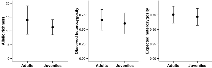
Fig. 5. Allelic richness, observed heterozygosity, and expected heterozygosity in adult and juvenile trees on Wattkast. Values represent the average across all loci ± s.d. Note that none of the differences was statistically significant (ANOVA, P > 0.05 for all panels A–C).