| Table 1. Main scenarios of the study. | |||
| First thinning removal | Min. top diameter of wood, cm | Moisture content, % | |
| Scenario 1 | industrial wood | 6 | 55 |
| Scenario 2 | delimbed energy wood | 4 | 35 |
| Scenario 3 | whole trees for energy | 0 | 45 |
| Table 2. Productivity (PMH15 = Productive machine hour excluding delays longer than 15 minutes), payload (m3 = solid cubic meter) and cost parameters (€ h–1) used in the study scenarios. | |||
| Average productivity (m3 h–1, PMH15) | Payload (m3) | Cost (€ h–1) | |
| Cutting | |||
| Scenario 1 | 8.2 m3 h–1 | 102.30 € h–1 | |
| Scenario 2 | 8.7 m3 h–1 | 102.30 € h–1 | |
| Scenario 3 | 9.7 m3 h–1 | 102.30 € h–1 | |
| Forwarding | |||
| Scenario 1 | 12.2 m3 h–1 | 11 m3 | 81.00 € h–1 |
| Scenario 2 | 12.1 m3 h–1 | 10 m3 | 81.00 € h–1 |
| Scenario 3 | 8.5 m3 h–1 | 6 m3 | 81.00 € h–1 |
| Truck transportation | |||
| Scenario 1 | 12.8 m3 h–1 (100 km) | 57 m3 | 72 € h–1 |
| Scenario 2 | 14.7 m3 h–1 (100 km) | 67 m3 | 72 € h–1 |
| Scenario 3 | 6.6 m3 h–1 (100 km) | 30 m3 | 66 € h–1 |
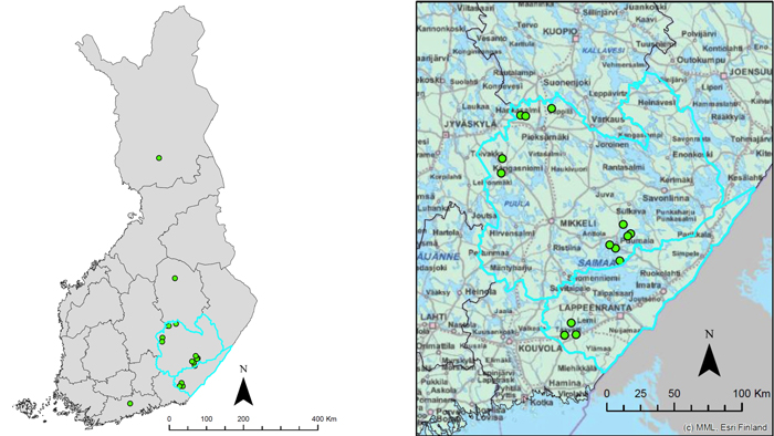
Fig. 1. The data points from the study, with highlighting for areas in the regional case of South Savo (and South Karelia) in eastern Finland.
| Table 3. Stand characteristics of plots in the alternative areas of Finland (‘Regional case’ = South Savo and South Karelia), with different stand density classes. N = number of stems per hectare, G = stand basal area (m2 ha–1), Dg = mean diameter at breast height (cm), Hg = mean height (m), T = age (years), and V = volume (m3). | ||||||||
| Area | Stand density class, N | Plot number | T | G | N | Dg | Hg | V |
| Regional case | < 3000 | 1 | 28 | 21.7 | 1140 | 16.8 | 13.8 | 149.7 |
| 2 | 25 | 21.3 | 1218 | 15.3 | 12.5 | 135.3 | ||
| 3 | 19 | 11.0 | 1847 | 9.4 | 7.6 | 46.9 | ||
| 4 | 17 | 17.8 | 1886 | 11.9 | 9.5 | 89.7 | ||
| 5 | 22 | 18.5 | 2240 | 11.2 | 9.6 | 95.0 | ||
| 6 | 17 | 9.2 | 2502 | 7.5 | 6.2 | 34.0 | ||
| 7 | 26 | 16.0 | 2515 | 9.7 | 9.3 | 80.1 | ||
| 8 | 33 | 29.7 | 2633 | 13.0 | 11.3 | 174.3 | ||
| 9 | 15 | 11.9 | 2802 | 8.6 | 6.8 | 46.8 | ||
| > 3000 | 10 | 16 | 11.1 | 3002 | 8.1 | 6.6 | 42.0 | |
| 11 | 35 | 36.8 | 3065 | 13.3 | 13.5 | 241.5 | ||
| 12 | 31 | 9.5 | 3803 | 6.9 | 7.9 | 41.8 | ||
| 13 | 13 | 10.7 | 4500 | 5.8 | 4.3 | 30.1 | ||
| 14 | 11 | 4.6 | 4900 | 3.5 | 4.2 | 13.7 | ||
| 15 | 34 | 30.8 | 4794 | 10.9 | 10.7 | 168.4 | ||
| southern Finland | 3000 | 16 | 23 | 12.7 | 3000 | 9.3 | 6.3 | 46.5 |
| central Finland | 3000 | 17 | 27 | 12.1 | 3000 | 9.2 | 6.0 | 43.4 |
| northern Finland | 3000 | 18 | 34 | 13.0 | 3000 | 9.5 | 6.2 | 47.1 |
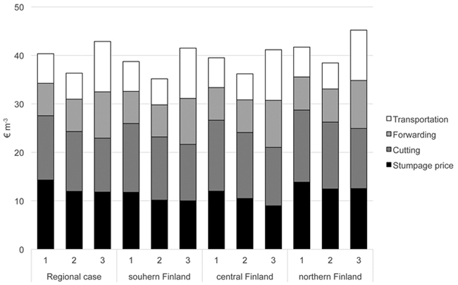
Fig. 2. Total supply-chain costs, in € m–3, with a transport distance of within 100 km (chipping cost is not included). Scenario 1: industrial wood, Scenario 2: delimbed energy wood, Scenario 3: whole trees for energy. ‘Regional case’ = South Savo (and South Karelia).
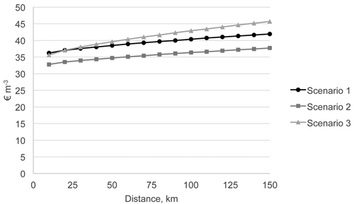
Fig. 3. Average supply-chain costs, in € m–3, in relation to distance in the regional case (South Savo and South Karelia) (chipping cost is not included).
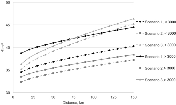
Fig. 4. Average total supply-chain costs in the regional case of South Savo (and South Karelia) (chipping cost is not included) plotted against distance and the density of the stand (>3000 trees ha–1 and <3000 trees/ha, in € m–3).
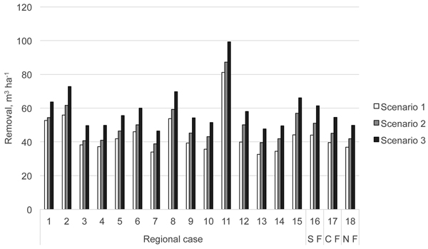
Fig. 5. Total first thinning removal of scenarios (Scenario 1: Industrial wood; Scenario 2: Delimbed energy wood; Scenario 3: Whole tree) and plots (plot number 1–18) in the regional case of South Savo (and South Karelia), and in the other regional areas of Finland (S F = southern Finland, 1300 dd., C F = central Finland, 1100 dd., N F = northern Finland, 900 dd.).
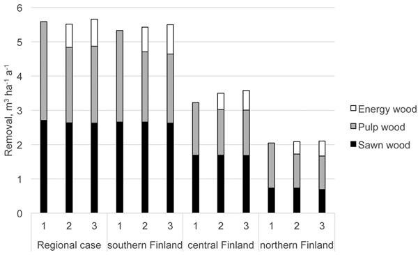
Fig. 6. Total annual removal of sawn wood, pulp wood, and energy wood from the whole forest rotation (m3 ha–1 a–1) in the alternative scenarios studied in the regional case of South Savo (and South Karelia), and in the other areas of Finland.
| Table 4. Estimated average stumpage prices for each scenario and area (‘Regional case’: = South Savo and South Karelia, ‘Regional areas’: ‘S F’ = southern Finland, ‘C F’ = central Finland, ‘N F’ = northern Finland). Minimum (min) and maximum (max) values of stumpage prices has been presented in the regional case. | ||||||
| Regional case | Regional areas | |||||
| mean | min | max | S F | C F | N F | |
| Scenario 1 | 14.3 | 14.0 | 16.4 | 11.7 | 12.0 | 13.9 |
| Scenario 2 | 12.0 | 6.8 | 15.9 | 10.1 | 10.5 | 12.4 |
| Scenario 3 | 11.8 | 7.7 | 15.4 | 10.0 | 9.0 | 12.6 |