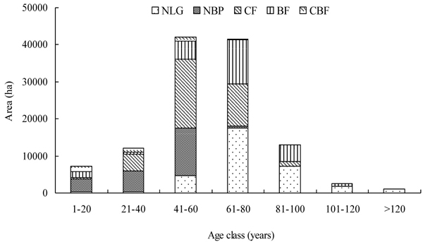
Fig. 1. The age class distribution of forest landscape dataset, where NLG = natural Larix gmelinii dominated forests, NBP = natural Betula platyphylla dominated forests, CF = coniferous forests, BF = broad-leaved forests, and CBF = coniferous and broad-leaved mixed forests.
| Table 1. The potential management prescriptions for the forest planning problems. | ||||
| No. | Management prescription | Limit age (year) | Description | |
| Broad-leaved forest a | Coniferous forest b | |||
| 0 | No harvest | < 20 | < 30 | Strictly prohibit any management prescriptions when stand age is less than the limiting ages |
| 1 | Mild selective cutting c | 21–50 | 31–80 | Only can adopt one of the three intensities of selective cutting, as well as no harvest, when stand age ranges within the interval of the limiting ages |
| 2 | Moderate selective cutting d | |||
| 3 | Severe selective cutting e | |||
| 4 | Final harvest | > 50 | > 80 | Can adopt final harvest, selective cutting and no harvest when forest age is more than the limiting ages |
| a include natural Betula platyphylla dominated forests (NBP) and broad-leaved forests (BF) b include natural Larix gmelinii dominated forests (NLG), coniferous forests (CF) and coniferous and broad-leaved mixed forests (CBF) c the intensity of selective cutting was assumed as 10% of the total volume for a management unit d the intensity of selective cutting was assumed as 20% of the total volume for a management unit e the intensity of selective cutting was assumed as 30% of the total volume for a management unit | ||||
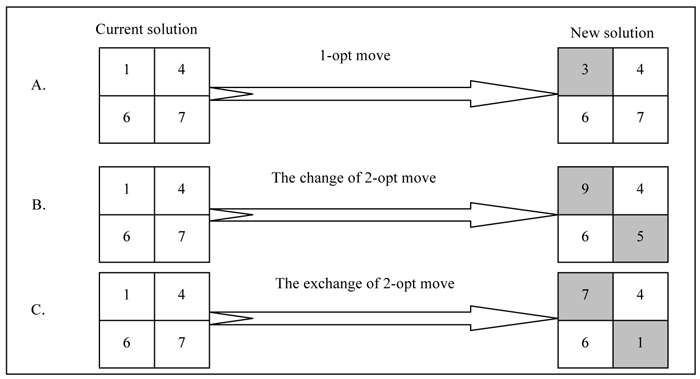
Fig. 2. The schematic diagram of different neighborhood search strategies of simulated annealing, where A is 1-opt moves, B is the change version of 2-opt moves, and C is the exchange version of 2-opt moves. The number in each cell represents the assigned harvest period.
| Table 2. Quality ((m3)2) of the best solutions (i.e., minimum solution values) generated with five different exchange rates (Methods 3 and 4) and reversion rates (Methods 5 and 6) for the forest spatial planning problem, where R2-R10 represent the five oscillation (or reversion) rates (i.e., R = 2, 4, 6, 8, 10). | |||||
| Method | Oscillation / reversion rate | ||||
| 2 | 4 | 6 | 8 | 10 | |
| 3 | 87.6 | 135.7 | 73.2 | 143.2 | 89.7 |
| 4 | 62.0 | 23.3 | 66.9 | 20.9 | 12.9 |
| 5 | 60.0 | 13.1 | 50.8 | 51.7 | 88.5 |
| 6 | 20.9 | 29.2 | 16.0 | 36.2 | 11.8 |
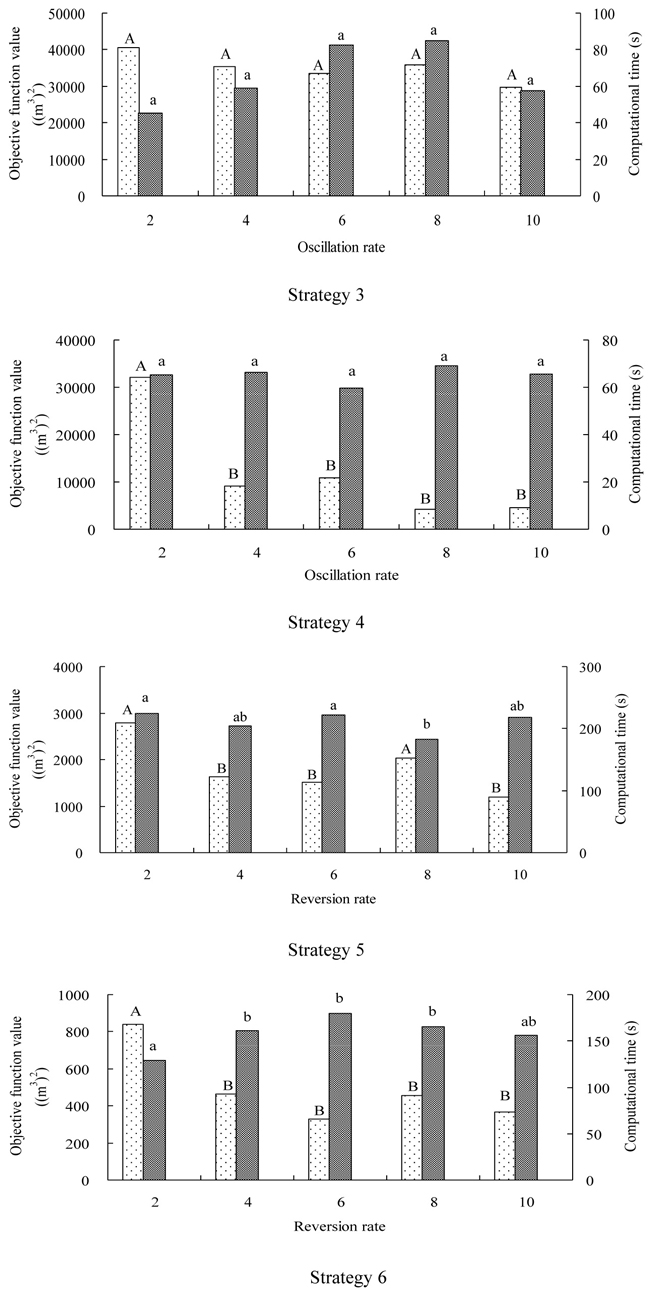
Fig. 3. The mean objective function values (dot-bar) and computational time (line-bar) required for the different oscillation rates (Strategies 3 and 4) and reversion rates (Strategies 5 and 6) for the forest spatial planning problem. The same upper-case letter in the dot-bar indicates that there are no significant differences in objective function values at α = 0.05 between different search strategies when implemented with simulated annealing algorithm. The same lower-case letter in the line-bar indicates that there are no significant differences in computational time at α = 0.05 between different search strategies when implemented with simulated annealing algorithm.
| Table 3. The statistical characteristics of objective function values and computational time of 60 independent solutions for the six alternative search strategies when implemented with simulated annealing algorithm. | ||||||||
| Search strategy | Objective function values (m3)2 | Computational time (seconds) | ||||||
| Minimum | Maximum | Mean | Standard deviation | ANOVA groups a | Mean | Standard deviation | ANOVA groups b | |
| 1 | 410.1 | 113 712.0 | 36 541.7 | 26 011.1 | A | 41.1 | 47.1 | a |
| 2 | 29.4 | 78 059.7 | 25 559.3 | 22 544.5 | B | 162.2 | 208.6 | b |
| 3 | 89.7 | 113 668.0 | 29 679.4 | 23 443.0 | B | 57.4 | 82.3 | a |
| 4 | 20.9 | 77 266.0 | 4138.2 | 9864.1 | C | 69.1 | 77.8 | a |
| 5 | 88.5 | 5867.5 | 1190.5 | 1413.1 | C | 218.3 | 89.8 | c |
| 6 | 16.0 | 1346.9 | 327.3 | 291.2 | C | 180.1 | 75.7 | bc |
| a The same letter indicate that there are no significant differences in objective function values at α = 0.05 between different search strategies when implemented with simulated annealing algorithm. b The same letter indicate that there are no significant differences in computational time at α = 0.05 between different search strategies when implemented with simulated annealing algorithm. | ||||||||
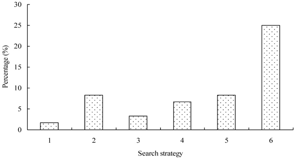
Fig. 4. The percentage of the sixty objective function values for each search strategy that varied within 10 times (i.e., ≤ 118.0 (m3)2) of the best solution value generated by Strategy 6 with a reversion interval of 10 iterations.
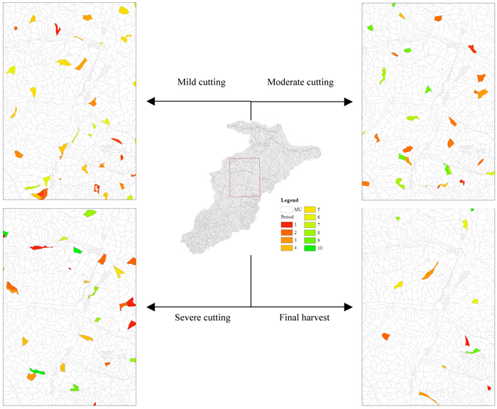
Fig. 5. The spatial and temporal assignment of management prescriptions of a small subarea for the best solution that generated by Strategy 6 with a reversion interval of 10 iterations, where MU is management unit. View larger in new window/tab.