| Table 1. Description of investigated provenances. | ||||||
| Ecotypes | No. of prov. | Provenance name | Altitude | Geographic coordinates | Age of adult stand | |
| latitude | longitude | |||||
| northern | 3 | Radachowo | 193 | 53°05´N | 15°54´E | 107 |
| 7 | Gniewino | 115 | 54°37´N | 18°18´E | 110 | |
| 8 | Jelenino | 130 | 53°40´N | 16°40´E | 96 | |
| 9 | Dalęcino | 130 | 53°45´N | 16°30´E | 111 | |
| 11 | Marianowo | 70 | 54°23´N | 18°31´E | 105 | |
| 17 | Mikołajki | 40 | 53°51´N | 19°10´E | 159 | |
| 19 | Tumiany | 175 | 53°58´N | 20°57´E | 130 | |
| southern | 31 | Pokrzywna | 425 | 50°20´N | 17°20´E | 130 |
| 34 | Jeleniów | 350 | 50°50´N | 20°59´E | 101 | |
| 37 | Marynin | 170 | 50°23´N | 22°17´E | 96 | |
| 39 | Bukowa | 550 | 49°39´N | 18°54´E | 122 | |
| 42 | Moczarna | 700–920 | 49°07´N | 22°29´E | 135 | |
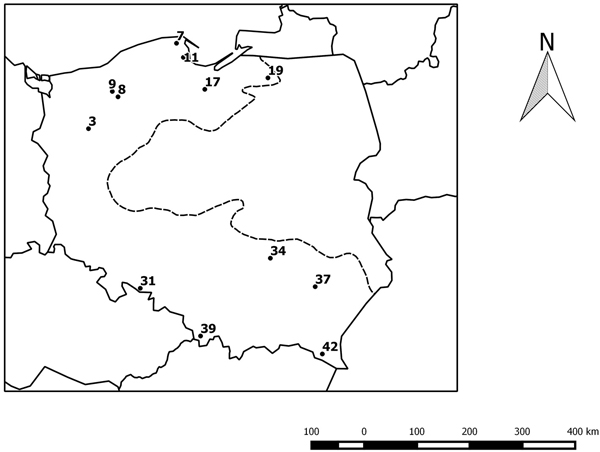
Fig. 1. Geographical distribution of the studied provenances. The black circles indicate the location of the beech provenances, see Table 1. The dotted line indicates the limit of the beech range in Poland.
| Table 2. Summary statistics for the 10 microsatellite loci. | |||||||||
| Locus | Size range (bp) | No. of alleles | NA | NE | HO | HE | FIS | FST | |
| csolf31 | 106–128 | 13 | 10.40 | 5.51 | 0.837 | 0.815 | –0.017 | 0.030 | |
| FS3-04 | 193–205 | 5 | 3.60 | 1.61 | 0.347 | 0.346 | 0.034 | 0.087 | |
| mfc11 | 321–355 | 12 | 7.70 | 4.03 | 0.738 | 0.739 | –0.010 | 0.040 | |
| FS1-15 | 92–146 | 23 | 9.80 | 5.52 | 0.762 | 0.813 | 0.055*** | 0.034 | |
| csolf19 | 151–181 | 12 | 9.70 | 4.87 | 0.795 | 0.789 | –0.004 | 0.032 | |
| mfs11 | 128–164 | 12 | 7.90 | 4.06 | 0.731 | 0.740 | 0.001 | 0.041 | |
| mfc7 | 111–173 | 15 | 5.90 | 2.13 | 0.526 | 0.501 | –0.045 | 0.040 | |
| mfc5 | 277–333 | 25 | 16.10 | 8.09 | 0.800 | 0.866 | 0.071*** | 0.037 | |
| sfc0036 | 97–111 | 8 | 7.10 | 4.13 | 0.758 | 0.747 | –0.013 | 0.030 | |
| DE576A0 | 219–240 | 7 | 5.30 | 2.92 | 0.683 | 0.651 | –0.040 | 0.037 | |
| Mean (overall) | - | 13.2 | 8.35 | 4.29 | 0.698 | 0.701 | 0.003 | 0.041 | |
| The size range: the minimum and maximum lengths of PCR product detected for a locus (in base pairs), NA – mean number of alleles, NE – effective number of alleles, HO – observed hetrozygosity, HE – expected hetrozygosity, FIS – inbreeding coefficient. Significance of FIS values: *** p<0.001 | |||||||||
| Table 3. Diversity measures in Fagus sylvatica. | |||||||||
| Ecotypes | Provenance | NA | NE | HO | HE | F | No. Private Alleles | Freq | |
| northern | 3 | Radachowo | 7.90 | 4.11 | 0.677 | 0.694 | 0.023 | 1 | 0.02 |
| 7 | Gniewino | 8.00 | 3.81 | 0.707 | 0.707 | –0.003 | 3 | 0.06 | |
| 8 | Jelenino | 7.70 | 4.49 | 0.679 | 0.698 | 0.025* | 1 | 0.02 | |
| 9 | Dalęcino | 7.80 | 4.32 | 0.707 | 0.710 | 0.010 | 1 | 0.01 | |
| 11 | Marianowo | 8.30 | 4.09 | 0.681 | 0.696 | 0.011 | 1 | 0.01 | |
| 17 | Mikołajki | 8.10 | 4.25 | 0.715 | 0.723 | 0.014* | 2 | 0.02 | |
| 19 | Tumiany | 8.00 | 4.39 | 0.715 | 0.717 | 0.017 | 1 | 0.01 | |
| Mean | 7.97 | 4.21 | 0.697 | 0.706 | 0.014 | 0.02 | |||
| southern | 31 | Pokrzywna | 9.00 | 4.88 | 0.679 | 0.696 | 0.038 | 3 | 0.03 |
| 34 | Jeleniów | 8.30 | 4.56 | 0.735 | 0.710 | –0.041* | 2 | 0.02 | |
| 37 | Marynin | 8.20 | 3.52 | 0.673 | 0.665 | –0.015* | 1 | 0.02 | |
| 39 | Bukowa | 9.20 | 4.60 | 0.750 | 0.730 | –0.041* | 6 | 0.13 | |
| 42 | Moczarna | 9.10 | 4.48 | 0.688 | 0.701 | 0.014 | 4 | 0.04 | |
| Mean | 8.76 | 4.41 | 0.705 | 0.701 | –0.009 | 0.05 | |||
| Mean | 8.30 | 4.29 | 0.701 | 0.704 | 0.004 | 0.03 | |||
| NA – mean number of alleles, NE – effective number of alleles, HO – observed heterozygosity, HE – expected heterozygosity, F – fixation index. Significance of F values: * p<0.01, number of private alleles and their frequency (Freq). | |||||||||
| Table 4. Hierarchical analysis of molecular variance (AMOVA) based on allelic distance matrix. | ||||||
| Variance component | df | SS | MS | Variance | % Total | P |
| Among Regions | 1 | 70.486 | 70.486 | 0.162 | 2% | 0.010 |
| Among Pops | 10 | 250.160 | 25.016 | 0.368 | 5% | 0.010 |
| Within Pops | 564 | 4134.229 | 7.330 | 7.330 | 93% | 0.010 |
| Total | 575 | 4454.875 | ||||
| df – degree of freedom, SS – Sum of squares, MS – Mean squares, P – probability | ||||||
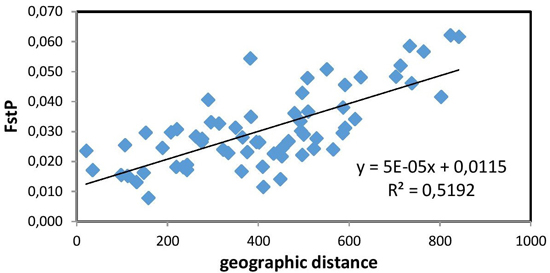
Fig. 2. Relationship between pairwise FST values and geographic distance (km) (R = 0.721, p = 0.01) between the studied 12 populations of European beech.
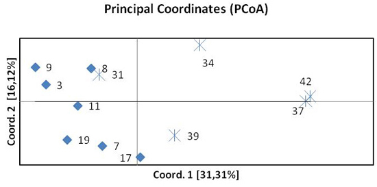
Fig. 3. Principal Coordinates Analysis (PCoA) of pairwise FST of twelve beech populations. Diamonds represent provenances from the north, crosses provenances from the south.
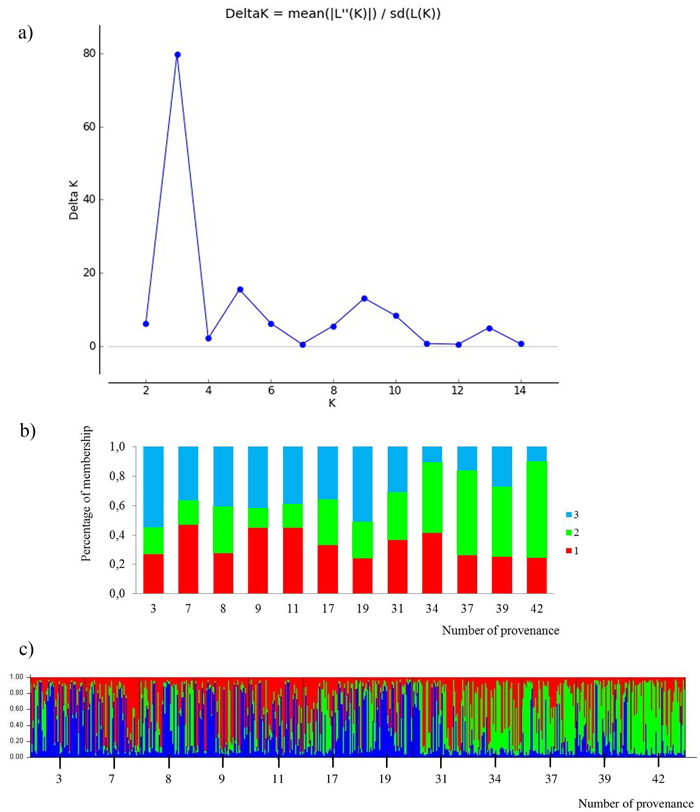
Fig. 4. Results for STRUCTURE analysis:
a) values of the statistic “Delta K” for all calculated K-values from 1–15 based on the combined dataset of nuclear microsatellites. The highest “Delta K” corresponds to the uppermost level of hierarchy among runs (Evanno et al. 2005).
b) proportion of membership of each individual to three assumed subpopulations (K = 3).
c) proportion of membership of each individual to three assumed subpopulations (K = 3). (Northern provenances: 3 to 19; Southern provenances 31 to 42. For location names see Table 3). View larger in new window/tab.