| Table 1. The location of the populations (culling sites) and the number of sampled individuals for the DNA marker study. Population ID is given in numeric and letter format. Zone is eco-climatic zone (considered as region in the ANOVA). N is the number of individuals. Eco is the ecotype (Fo – forest ecotype population; Fld – field ecotype). | ||||||
| Pop id | Pop id | Zone | N | Eco | Latitude, Longitude | Culling location |
| ADE | 1 | I | 2 | Fo | 23°02´N, 55°48´E | Siauliai region, Kurtuvenu National Park, Naisiai |
| PLA | 2 | I | 3 | Fo | 21°53´N, 56°01´E | Plunge region, Plokstine forest |
| SIA | 3 | I | 3 | Fo | 23°22´N, 55°48´E | Siauliai region, Pakape forest |
| JON | 4 | II | 12 | Fld | 23°42´N, 56°16´E | Joniskis region |
| RAD | 5 | II | 8 | Fo | 23°29´N, 55°32´E | Radviliskis region, Bargailiai forest |
| NID | 6 | III | 4 | Fo | 21°01´N, 55°21´E | Neringa region, Briedziu forest |
| SIL | 7 | III | 9 | Fld | 21°21´N, 55°20´E | Silute region |
| ALY | 8 | IV | 3 | Fo | 23°58´N, 54°26´E | Alytus region |
| GIR | 9 | IV | 10 | Fo | 24°04´N, 54°49´E | Kaunas region, Dubrava forest |
| KAM | 10 | IV | 9 | Fld | 23°47´N, 54°54´E | Kaunas region, Kamsa forest |
| PRI | 12 | IV | 3 | Fo | 23°54´N, 54°36´E | Prienai region, Prienu Silas forest |
| VIR | 13 | IV | 13 | Fld | 22°48´N, 54°35´E | Vilkaviskis region, Virbalgiris forest and surrounding fields |
| Total | 79 | |||||
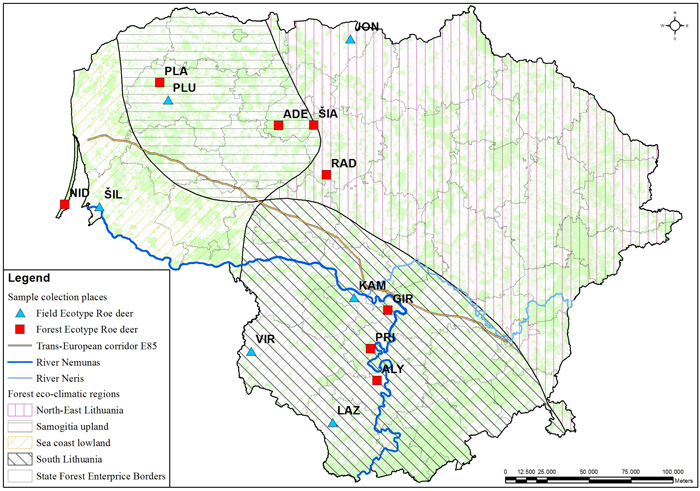
Fig. 1. Culling location of the sampled roe deer populations. The populations with field or forest ecotypes are indicated with different markers. Abbreviations explained in Table 1. The lines delineate the eco-climatic zones. The outlined populations were used for the DNA marker study. The populations marked in the map indicates the culling location. View larger in new window/tab.
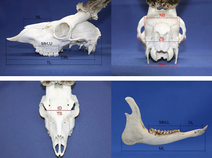
Fig. 2. Roe deer skull morphometry traits. View from the left side; NL – nasal length, MtrLU – maxilla tooth row length, CBL – condylobasal length, TL – total length of skull. View from the back side; NB – neurocranium breadth, ZB – zigomatic breadth, Mw – mastoidic width. View from the top; ID – interorbital distance, TB – total breadth. View from the right side of lower jaw; ML – Mandible length, MtrLL – mandible tooth raw length, DL – diastema length, Sm – the height of second molar tooth.
| Table 2. The loci mean statistics (the standard error is given in the parenthesis, except for FST and RST for which the p values are given). The RST, FST differentiation is among roe deer populations. Na is total number of different alleles. Ne is the effective number of alleles He is expected heterozygosity (uHe is unbiased He corrected for sample size differences). FIS is inbreeding coefficient, RST and FST are the genetic differentiation indexes based on stepwise and infinitesimal mutation models. | |||||
| Index | N30 | N71 | N48 | N16 | N24 |
| Na | 3 | 9 | 7 | 11 | 11 |
| Ne | 2.01 (0.01) | 3.02 (0.31) | 3.70 (0.36) | 3.80 (0.50) | 2.60 (0.18) |
| Ho | 0.90 (0.05) | 0.73 (0.06) | 0.72 (0.07) | 0.64 (0.02) | 0.98 (0.02) |
| He | 0.50 (0.00) | 0.66 (0.03) | 0.72 (0.03) | 0.72 (0.03) | 0.61 (0.61) |
| uHe | 0.52 (0.00) | 0.68 (0.03) | 0.75 (0.04) | 0.75 (0.03) | 0.63 (0.03) |
| FIS | –0.79 (0.10) | –0.13 (0.13) | 0.01 (0.07) | 0.11 (0.06) | –0.62 (0.05) |
| RST | 0.051 (0.032) | 0.019 (0.153) | 0.088 (0.007) | 0.102 (0.004) | 0.068 (0.018) |
| FST | –0.019 (0.859) | –0.011 (0.778) | 0.032 (0.019) | 0.018 (0.057) | –0.007 (0.634) |
| Table 3. The differentiation indexes among the field and forest ecotypes based on AMOVA. | ||||||
| Index | N30 | N71 | N48 | N16 | N24 | Total |
| RST | 0.060 | –0.004 | –0.012 | –0.013 | –0.007 | 0.003 |
| p value (rand> = data) | 0.010 | 0.448 | 0.738 | 0.999 | 0.511 | 0.265 |
| FST | –0.005 | 0.027 | –0.002 | –0.007 | –0.009 | 0.001 |
| p value (rand> = data) | 0.462 | 0.028 | 0.483 | 0.803 | 0.859 | 0.334 |
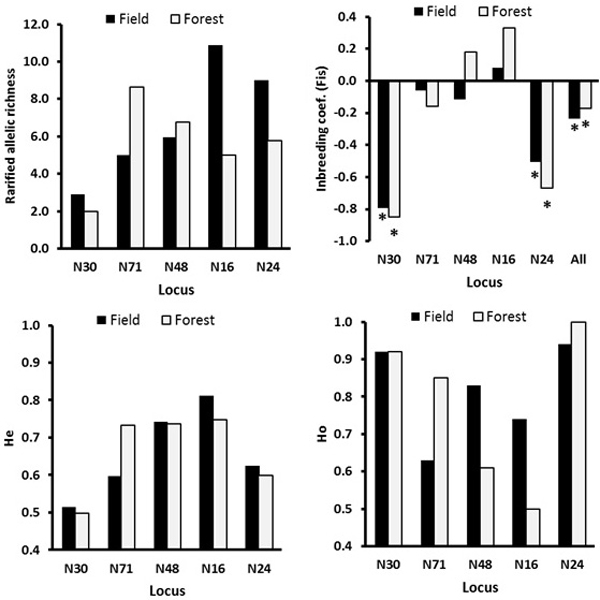
Fig. 3. The locus-wise genetic diversity parameters compared between the field and the forest ecotypes calculated with FSTAT software. For the inbreeding coefficient, the multilocus estimate was calculated (“all” on the X-axis, upper right plot). The asterisks mark the FIS values significant at the 0.05 level as estimated over 200 randomizations, based on the proportion of the randomizations that gave smaller or larger value than the observed value, so indicating significantly negative or positive FIS values.
| Table 4. Comparison of the multi loci genetic diversity parameters among the sexes within the field and forest ecotypes. N is the number of individuals. SE is standard error. The genetic diversity parameters are explained in Table 2. | ||||||||
| Ecotype/gender | Stat. | N | Na | Ne | Ho | He | uHe | FIS |
| Field/Female | Mean | 15.8 | 5.40 | 3.23 | 0.79 | 0.64 | 0.66 | –0.30 |
| SE | 1.20 | 0.68 | 0.06 | 0.05 | 0.06 | 0.18 | ||
| Forest/Female | Mean | 24.8 | 5.40 | 3.13 | 0.79 | 0.65 | 0.67 | –0.26 |
| SE | 1.10 | 0.37 | 0.07 | 0.04 | 0.04 | 0.20 | ||
| Field/Male | Mean | 20.2 | 5.20 | 3.09 | 0.82 | 0.65 | 0.66 | –0.29 |
| SE | 1.10 | 0.40 | 0.07 | 0.04 | 0.04 | 0.15 | ||
| Forest/Male | Mean | 13.6 | 4.20 | 2.89 | 0.72 | 0.63 | 0.65 | –0.22 |
| SE | 0.70 | 0.33 | 0.13 | 0.04 | 0.04 | 0.28 | ||
| Table 5. The multilocus mean within population (culling location) genetic diversity indexes. The eco-climatic zone is given in the parenthesis at the population name. N is the number of individuals. Data for populations with sample size > = 4 are shown. | ||||||
| Pop (eco climatic zone) | N | Na | Ne | Ho | uHe | FIS |
| JON (2) | 12 | 4.80 | 3.00 | 0.80 | 0.67 | –0.27 |
| RAD (2) | 8 | 3.80 | 3.03 | 0.90 | 0.69 | –0.44 |
| NID (3) | 4 | 3.40 | 2.77 | 0.73 | 0.71 | –0.20 |
| SIL (3) | 9 | 3.60 | 2.72 | 0.78 | 0.65 | –0.33 |
| GIR (4) | 10 | 3.00 | 2.54 | 0.69 | 0.63 | –0.23 |
| KAM (4) | 10 | 4.00 | 2.53 | 0.71 | 0.61 | –0.24 |
| PRI (4) | 12 | 2.80 | 2.31 | 0.73 | 0.67 | –0.35 |
| VIR (4) | 13 | 4.80 | 3.33 | 0.87 | 0.69 | –0.36 |
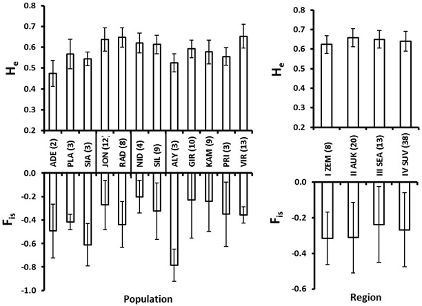
Fig. 4. Roe deer culling location (population, left) and eco-climatic zone (region, right) mean and standard error values for expected heterozygosity (He) and the inbreeding coefficient (FIS). Number of individuals in each population and region is given in the parenthesis at the abbreviations of the populations (culling locations), which are explained in Table 2. The vertical lines at the X-axis in the left plot delineate regions (eco-climatic zones).
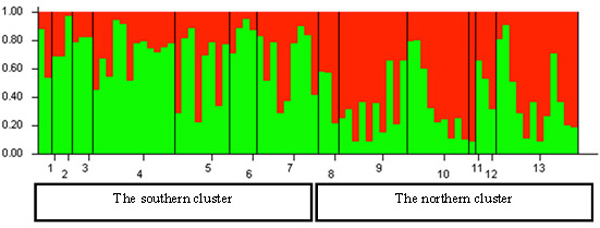
Fig. 5. Histogram of genetic structure of roe deer in Lithuania based on Bayesian clustering with STRUCTURE software. The two colours represent different STRUCTURE clusters. Populations are separated by vertical lines and identified on the X-axis by numbers (pop id in Table 1), where larger sample sizes correspond to longer intervals on the X-axis (each individual is a separate colour line). Y-axis is the likelihood for the individual membership into each of the two clusters separated by the STRUCTURE software and indicated here with different colour. The southern cluster includes individuals sampled in southern Lithuania and seacost lowland eco-climatic zones. The northern cluster includes individuals sampled in northeastern Lithuania and Samogitia upland.
| Table 6. The mean value and the variance of roe deer skull morphology traits, given by three age classes. Age class 1st (age from 0 to 1 years), age class 2 (age from 2 years to 3 years), age class 3 (age from 3 years to 10 years). M is a mean value, N is the number of individuals, CV is a coefficient of variance, Min and Max is a minimal and maximal values. The abbreviations of the traits are explained in Fig. 2. | |||||||||||||||
| Variable | AGE CLASS = 1 | AGE CLASS = 2 | AGE CLASS = 3 | ||||||||||||
| M | N | CV | Min | Max | M | N | CV | Min | Max | M | N | CV | Min | Max | |
| TLENGHT | 18.2 | 110 | 4.9 | 16.2 | 20.9 | 19.8 | 32 | 3.2 | 18.6 | 21.0 | 20.4 | 388 | 3.4 | 18.6 | 22.3 |
| CLENGHT | 17.1 | 110 | 4.8 | 15.4 | 19.6 | 18.7 | 32 | 3.7 | 17.5 | 20.0 | 19.3 | 385 | 3.4 | 17.5 | 21.2 |
| TBREADTH | 8.1 | 118 | 5.1 | 7.2 | 9.0 | 8.9 | 40 | 3.7 | 8.2 | 9.6 | 9.3 | 445 | 4.7 | 7.8 | 10.6 |
| ORBDIST | 4.9 | 118 | 8.5 | 4.3 | 7.2 | 5.3 | 40 | 6.5 | 4.6 | 6.7 | 5.5 | 445 | 6.5 | 4.5 | 6.9 |
| ZBREADTH | 6.5 | 116 | 9.9 | 4.9 | 8.2 | 7.2 | 40 | 7.7 | 6.3 | 8.8 | 7.4 | 443 | 8.5 | 5.2 | 9.0 |
| NASALONG | 5.0 | 108 | 9.0 | 3.9 | 7.0 | 5.8 | 39 | 7.2 | 5.0 | 6.6 | 5.9 | 432 | 8.4 | 4.5 | 7.2 |
| NEURLONG | 5.7 | 117 | 3.6 | 5.3 | 6.2 | 5.9 | 40 | 3.6 | 5.4 | 6.4 | 6.1 | 442 | 3.8 | 5.4 | 6.7 |
| MTOOTR | 5.2 | 108 | 7.1 | 4.4 | 6.3 | 5.9 | 34 | 4.7 | 5.1 | 6.4 | 5.7 | 353 | 4.4 | 5.1 | 6.5 |
| MATOOTR | 5.6 | 114 | 10.1 | 4.5 | 7.0 | 6.6 | 39 | 4.5 | 6.1 | 7.2 | 6.5 | 361 | 4.3 | 3.9 | 7.4 |
| DIASTEM | 3.7 | 113 | 7.6 | 3.0 | 4.5 | 4.1 | 39 | 7.7 | 3.4 | 5.2 | 4.4 | 414 | 7.7 | 3.2 | 5.6 |
| MANDIBL | 14.2 | 113 | 5.6 | 12.4 | 16.3 | 15.5 | 38 | 3.7 | 14.6 | 16.8 | 16.0 | 395 | 3.5 | 13.7 | 17.2 |
| MASTOTIC | 4.3 | 89 | 6.7 | 3.6 | 5.0 | 4.5 | 35 | 8.7 | 3.7 | 6.1 | 4.6 | 263 | 8.0 | 3.7 | 5.7 |
| M2H | 0.7 | 70 | 16.4 | 0.4 | 0.8 | 0.7 | 35 | 10.4 | 0.5 | 0.9 | 0.6 | 340 | 19.4 | 0.2 | 0.9 |
| Trait abbreviations (see also Fig. 2); TBREADTH is total skull breadth, CLENGHT is total skull length, ORBDIST is interorbital distance, ZBREADTH is zigomatic breadth, NASALONG is nasal length, NEURLONG is a neurocranium length, MTOOTR is a maxilla tooth row length, MATOOTR is a mandible tooth row length, DIASREM is a diastema length, | |||||||||||||||
| Table 7. The results of ANOVA on the effect of the eco-climatic zone on roe deer skull morphometry run separately for male and female individuals and age class. DF for error by age class 1, 2, 3 (males) = 55, 31, 351; DF for error female = 55; 3; 85. F is the Fisher’s criterion and p > F is the significance of F from the ANOVA. The abbreviations of the traits are explained in Fig. 2. Bold values indicates a significant variance in particular traits and age classes. | ||||||
| AGE CLASS | NAME | DF | Males | Females | ||
| F | p > F | F | p > F | |||
| 1 | TLENGHT | 3 | 2.7 | 0.0575 | 1.8 | 0.1665 |
| 2 | TLENGHT | 3 | 0.5 | 0.6824 | 0.2 | 0.7172 |
| 3 | TLENGHT | 3 | 3.4 | 0.0189 | 0.3 | 0.8042 |
| 1 | CLENGHT | 3 | 2.9 | 0.0455 | 2.5 | 0.0707 |
| 2 | CLENGHT | 3 | 0.8 | 0.4982 | 1.0 | 0.3895 |
| 3 | CLENGHT | 3 | 5.2 | 0.0016 | 0.0 | 0.9908 |
| 1 | TBREADTH | 3 | 2.9 | 0.0409 | 1.6 | 0.1965 |
| 2 | TBREADTH | 3 | 1.9 | 0.1586 | 2.8 | 0.1926 |
| 3 | TBREADTH | 3 | 1.3 | 0.2835 | 0.6 | 0.6415 |
| 1 | ORBDIST | 3 | 1.4 | 0.2645 | 1.4 | 0.2389 |
| 2 | ORBDIST | 3 | 0.9 | 0.4525 | 2.0 | 0.2530 |
| 3 | ORBDIST | 3 | 0.5 | 0.6953 | 0.2 | 0.8741 |
| 1 | ZBREADTH | 3 | 2.7 | 0.0540 | 0.2 | 0.8817 |
| 2 | ZBREADTH | 3 | 0.1 | 0.9371 | 1.0 | 0.3937 |
| 3 | ZBREADTH | 3 | 6.5 | 0.0003 | 2.9 | 0.0418 |
| 1 | NASALONG | 3 | 4.3 | 0.0087 | 0.1 | 0.9383 |
| 2 | NASALONG | 3 | 1.2 | 0.3175 | 4.0 | 0.1397 |
| 3 | NASALONG | 3 | 0.9 | 0.4467 | 0.1 | 0.9424 |
| 1 | NEURLONG | 3 | 0.3 | 0.8008 | 2.5 | 0.0711 |
| 2 | NEURLONG | 3 | 1.0 | 0.4208 | 1.3 | 0.3357 |
| 3 | NEURLONG | 3 | 2.9 | 0.0342 | 0.9 | 0.4503 |
| 1 | MTOOTR | 3 | 2.5 | 0.0721 | 5.3 | 0.0029 |
| 2 | MTOOTR | 3 | 1.6 | 0.2168 | 0.6 | 0.4912 |
| 3 | MTOOTR | 3 | 9.5 | 0.0000 | 0.1 | 0.9839 |
| 1 | MATOOTR | 3 | 9.9 | 0.0000 | 1.8 | 0.1555 |
| 2 | MATOOTR | 3 | 1.6 | 0.2002 | 0.3 | 0.6134 |
| 3 | MATOOTR | 3 | 2.9 | 0.0345 | 5.2 | 0.0025 |
| 1 | DIASTEM | 3 | 4.8 | 0.0052 | 0.5 | 0.7178 |
| 2 | DIASTEM | 3 | 1.0 | 0.4016 | 2.8 | 0.1938 |
| 3 | DIASTEM | 3 | 19.1 | 0.0000 | 0.4 | 0.7203 |
| 1 | MANDIBL | 3 | 6.5 | 0.0008 | 1.7 | 0.1879 |
| 2 | MANDIBL | 3 | 0.7 | 0.5563 | 0.2 | 0.6737 |
| 3 | MANDIBL | 3 | 0.6 | 0.6263 | 0.4 | 0.7831 |
| 1 | MASTOTIC | 3 | 0.7 | 0.5426 | 0.4 | 0.7789 |
| 2 | MASTOTIC | 3 | 0.1 | 0.9565 | 0.1 | 0.8074 |
| 3 | MASTOTIC | 3 | 0.2 | 0.8903 | 1.2 | 0.3002 |
| 1 | M2H | 3 | 0.5 | 0.6877 | 1.2 | 0.3326 |
| 2 | M2H | 3 | 2.3 | 0.1061 | 0.0 | 0.9205 |
| 3 | M2H | 3 | 2.1 | 0.0966 | 1.2 | 0.3112 |
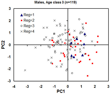
Fig. 6. Plot of individual principal component (PC) scores against the first pair of the PC from the principal component analysis for the male individuals of age class 3 (adults). Each eco-climatic zone (“Reg” on the plot) is marked with different markers. 1 is Samogitia upland, 2 is northeastern Lithuania, 3 is seaside lowland, 4 is southern Lithuania. The regional mean standard error for PC1 and PC2 scores is 1.5 and 2.0, respectively (to be used as an estimate of least significant difference). A tendency for higher PC1 scores of the northern regions 1 and 2 (meaning greater skull dimensions) is observed.
| Table 8. Results of ANOVA on the ecotype effect run separately for each age class. N is the number of roe deer individuals, SE is the standard error. F is the Fisher’s criterion and p is the significance of F from the ANOVA. The abbreviations of the variables are explained in Fig 2. Bold values indicates a significant variance in particular traits and age classes. | |||||||||
| Age class | Variable | ECOTYPE = Field | ECOTYPE = Forest | F | p > F | ||||
| Mean | N | SE | Mean | N | SE | ||||
| 1 | TLENGHT | 18.3 | 41 | 0.16 | 18.1 | 69 | 0.10 | 1.2 | 0.2813 |
| 2 | TLENGHT | 19.7 | 19 | 0.15 | 19.9 | 13 | 0.17 | 0.5 | 0.4744 |
| 3 | TLENGHT | 20.5 | 154 | 0.06 | 20.4 | 234 | 0.04 | 1.2 | 0.2675 |
| 1 | CLENGHT | 17.2 | 41 | 0.15 | 17.1 | 69 | 0.09 | 0.8 | 0.3631 |
| 2 | CLENGHT | 18.5 | 19 | 0.16 | 18.9 | 13 | 0.18 | 2.1 | 0.1586 |
| 3 | CLENGHT | 19.3 | 154 | 0.06 | 19.2 | 231 | 0.04 | 1.2 | 0.2814 |
| 1 | TBREADTH | 8.1 | 42 | 0.07 | 8.1 | 76 | 0.04 | 0.0 | 0.9134 |
| 2 | TBREADTH | 8.9 | 23 | 0.08 | 8.8 | 17 | 0.07 | 0.5 | 0.4829 |
| 3 | TBREADTH | 9.3 | 173 | 0.03 | 9.3 | 272 | 0.03 | 0.0 | 0.8798 |
| 1 | ORBDIST | 4.8 | 42 | 0.05 | 4.9 | 76 | 0.05 | 3.1 | 0.0804 |
| 2 | ORBDIST | 5.3 | 23 | 0.05 | 5.3 | 17 | 0.11 | 0.0 | 0.9958 |
| 3 | ORBDIST | 5.5 | 173 | 0.03 | 5.5 | 272 | 0.02 | 1.3 | 0.2552 |
| 1 | ZBREADTH | 6.5 | 42 | 0.12 | 6.5 | 74 | 0.07 | 0.0 | 0.8367 |
| 2 | ZBREADTH | 7.4 | 23 | 0.12 | 7.0 | 17 | 0.10 | 7.1 | 0.0110 |
| 3 | ZBREADTH | 7.4 | 172 | 0.05 | 7.4 | 271 | 0.04 | 0.1 | 0.7841 |
| 1 | NASALONG | 5.0 | 40 | 0.07 | 5.0 | 68 | 0.06 | 0.2 | 0.6909 |
| 2 | NASALONG | 5.8 | 23 | 0.09 | 5.8 | 16 | 0.11 | 0.0 | 0.9381 |
| 3 | NASALONG | 5.9 | 166 | 0.04 | 5.9 | 266 | 0.03 | 0.5 | 0.4674 |
| 1 | NEURLONG | 5.7 | 42 | 0.03 | 5.7 | 75 | 0.02 | 0.0 | 0.9298 |
| 2 | NEURLONG | 5.9 | 23 | 0.04 | 6.0 | 17 | 0.05 | 0.2 | 0.6366 |
| 3 | NEURLONG | 6.1 | 173 | 0.02 | 6.1 | 269 | 0.01 | 0.6 | 0.4456 |
| 1 | MTOOTR | 5.3 | 41 | 0.08 | 5.2 | 67 | 0.03 | 1.3 | 0.2547 |
| 2 | MTOOTR | 5.9 | 23 | 0.05 | 5.7 | 11 | 0.08 | 5.0 | 0.0331 |
| 3 | MTOOTR | 5.7 | 170 | 0.02 | 5.7 | 183 | 0.02 | 2.5 | 0.1163 |
| 1 | MATOOTR | 5.7 | 40 | 0.10 | 5.6 | 74 | 0.06 | 0.6 | 0.4413 |
| 2 | MATOOTR | 6.6 | 22 | 0.06 | 6.5 | 17 | 0.08 | 1.0 | 0.3304 |
| 3 | MATOOTR | 6.5 | 150 | 0.02 | 6.5 | 211 | 0.02 | 0.9 | 0.3336 |
| 1 | DIASTEM | 3.8 | 41 | 0.04 | 3.7 | 72 | 0.03 | 2.5 | 0.1148 |
| 2 | DIASTEM | 4.0 | 22 | 0.07 | 4.2 | 17 | 0.07 | 3.0 | 0.0919 |
| 3 | DIASTEM | 4.3 | 164 | 0.02 | 4.4 | 250 | 0.02 | 4.6 | 0.0328 |
| 1 | MANDIBL | 14.2 | 41 | 0.14 | 14.1 | 72 | 0.09 | 0.2 | 0.6535 |
| 2 | MANDIBL | 15.3 | 21 | 0.13 | 15.6 | 17 | 0.12 | 2.3 | 0.1394 |
| 3 | MANDIBL | 16.0 | 162 | 0.04 | 16.0 | 233 | 0.04 | 0.1 | 0.8139 |
| 1 | MASTOTIC | 4.2 | 32 | 0.04 | 4.3 | 57 | 0.04 | 3.4 | 0.0672 |
| 2 | MASTOTIC | 4.6 | 21 | 0.09 | 4.4 | 14 | 0.09 | 1.6 | 0.2179 |
| 3 | MASTOTIC | 4.7 | 125 | 0.03 | 4.6 | 138 | 0.03 | 2.9 | 0.0907 |
| 1 | M2H | 0.6 | 28 | 0.02 | 0.7 | 42 | 0.01 | 0.6 | 0.4427 |
| 2 | M2H | 0.7 | 19 | 0.02 | 0.7 | 16 | 0.02 | 0.0 | 0.9472 |
| 3 | M2H | 0.6 | 134 | 0.01 | 0.6 | 206 | 0.01 | 0.0 | 0.9703 |
| Table 9. The comparison of male roe deer antler traits among the age classes. F is the ANOVA Fisher’s criterion and p is the significance of F from the ANOVA with age as class the independent variable. SE is standard error. | |||||||||
| Age class (number of individuals) | Length of right buck, cm | Length of left buck, cm | Diameter of pedicle, cm | Circumstance of pedicle, cm | Circumstance of roses, cm | Diameter of roses, cm | Weight, g | Span between bucks, cm | |
| F | 38.4 | 37.5 | 28.0 | 29.9 | 15.9 | 25.9 | 28.6 | 10.7 | |
| p > F | 0.0001 | <0.0001 | <0.0001 | <0.0001 | <0.0001 | <0.0001 | <0.0001 | <0.0001 | |
| Age class 1 n = 15 | Mean | 11.81 | 11.99 | 1.50 | 4.82 | 13.30 | 5.06 | 186.72 | 5.20 |
| SE | 1.0 | 1.0 | 0.1 | 0.2 | 1.1 | 0.4 | 21.5 | 0.9 | |
| Age class 2 n = 32 | Mean | 14.41 | 14.56 | 1.71 | 5.42 | 15.32 | 5.76 | 255.76 | 7.54 |
| SE | 0.7 | 0.7 | 0.06 | 0.2 | 0.8 | 0.2 | 14.8 | 0.6 | |
| Age class 3 n = 83 | Mean | 18.57 | 18.52 | 1.90 | 6.01 | 15.90 | 6.44 | 294.91 | 8.56 |
| SE | 0.4 | 0.4 | 0.03 | 0.1 | 0.4 | 0.1 | 8.5 | 0.4 | |
| Age class 4 n = 52 | Mean | 21.57 | 21.68 | 2.15 | 6.86 | 19.09 | 7.34 | 365.60 | 10.05 |
| SE | 0.6 | 0.6 | 0.04 | 0.1 | 0.6 | 0.2 | 10.3 | 0.5 | |
| Age class 5 n = 110 | Mean | 21.45 | 21.59 | 2.23 | 6.96 | 19.28 | 7.76 | 357.3 | 10.10 |
| SE | 0.4 | 0.4 | 0.0 | 0.1 | 0.4 | 0.1 | 7.5 | 0.3 | |