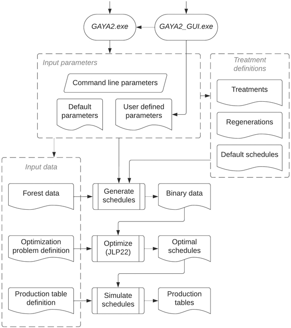
Fig. 1. Software system overview of the GAYA 2.0 forest stand simulator.

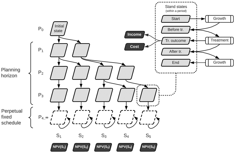
Fig. 2. Simulation procedure in GAYA 2.0. After the planning horizon, the silvicultural cycle is finalized according to the fixed schedule and the development stage. Beyond this, the fixed schedule is assumed to be applied cyclically forever. Periods are denoted P1, P2, etc., and schedules S1, S2, etc. NPV(S_i) denotes the net present value of the i-th schedule.

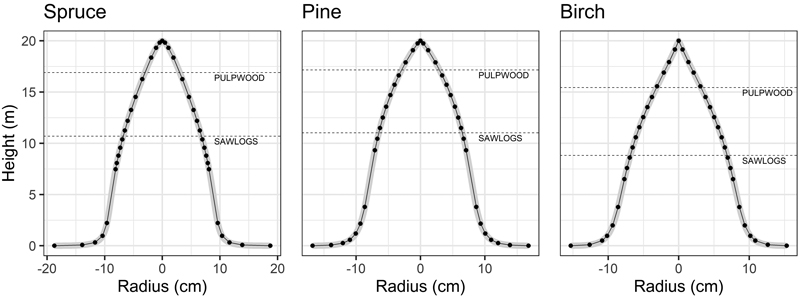
Fig. 3. GAYA 2.0 uses taper models to predict tree stem volume and its utilization with high precision. The trees in the example are 20 m in height and have a diameter at breast height of 20 cm. Pulpwood and sawlog heights correspond to minimum top diameters of 5 and 12 cm for pulpwood and sawlog, respectively. Dots mark the height location that minimize volume errors when approximating the volume of revolution of the tree stem. The tree species are Norway spruce (Picea abies), Scots pine (Pinus sylvestris), and birch (Betula pendula and B. pubescens).

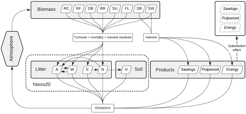
Fig. 4. The carbon cycle model in GAYA 2.0. The tree components are stem wood (SW), branches (BR), dead branches (DB), bark (SB), stump (SU), foliage (FL), fine roots (RF), and coarse roots (RC). The Yasso20 chemical compartments are celluloses (A), sugars (W), wax-like compounds (E), lignin-like compounds (N), and humus (H).

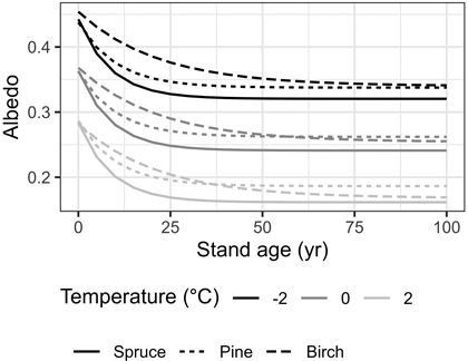
Fig. 5. GAYA 2.0 predicts forest surface albedo using the model in Bright et al. (2013). Here we illustrate albedo’s dependence on the mean annual temperature and stand age for the three species: Norway spruce (Picea abies), Scots pine (Pinus sylvestris), and birch (Betula pendula and B. pubescens).

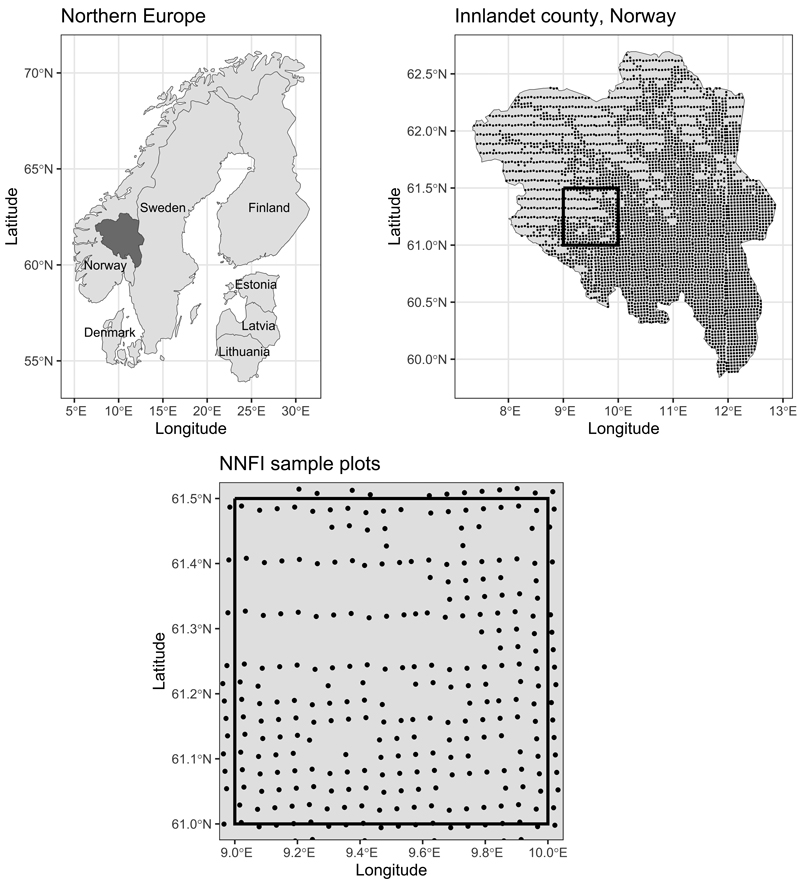
Fig. 6. The case study was conducted in Innlandet county in Norway. The approximative Norwegian National Forest Inventory (NNFI) plot locations are marked with dots. The apparent scattered plot positions are due to the random errors attached by NNFI to the coordinates when sharing plot data.

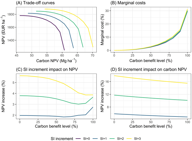
Fig. 7. GAYA 2.0 case study results. A – the trade-off curve between the net present value (NPV) and carbon NPV; B – marginal costs of different carbon benefit levels, expressed as percentage of the maximum NPV; C, D – impact of site index (SI) increments on NPV and carbon NPV, expressed as percentage increase from the base scenario SI+0.

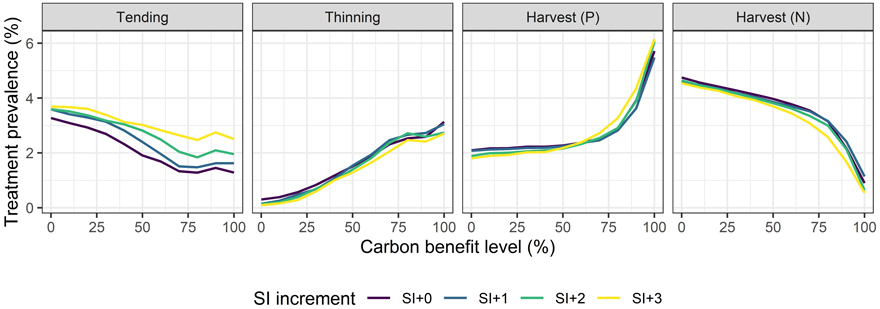
Fig. 8. GAYA 2.0 case study results. Treatment prevalence for tending, thinning, and harvest followed by planted (P), or natural (N) regeneration. The treatment prevalence is expressed as percentage of the area where the treatment was applied, averaged over the ten periods.

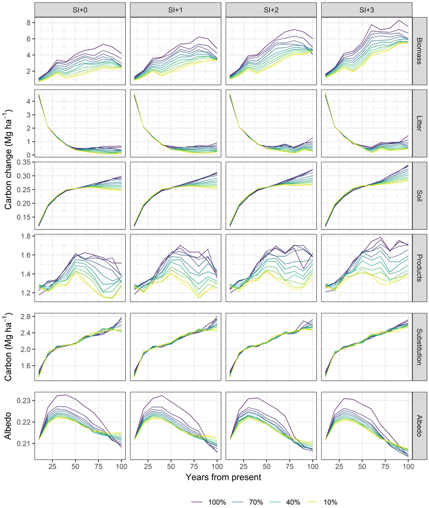
Fig. 9. GAYA 2.0 case study results. Predicted carbon changes by pool, substitution effect, and albedo over the planning horizon.

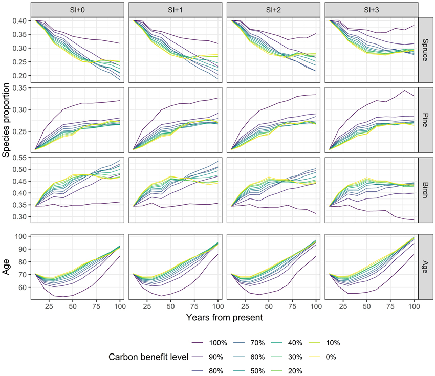
Fig. 10. GAYA 2.0 case study results. Changes in species composition and mean stand age over the planning horizon.