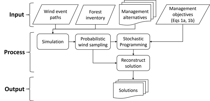
Fig. 1. Workflow of the study including the input information about wind, forest, and management and the modelling process used to find the final solutions.
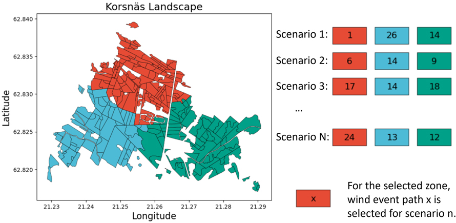
Fig. 2. A representation of the creation of the set of wind scenarios. For each zone, a wind event path (a set of wind events at varying intensities across the planning horizon) is selected, with a single landscape-level wind scenario being a combination of wind event paths for each zone.
| Table 1. Allocation scheme that assigns wind event paths into a specific group that represents a specific set of intensities and frequencies. A wind event path is a set of wind events at varying intensities across the planning horizon. The five groups represent different assumptions of wind disturbance patterns: low intensity low frequency (LL), low intensity and high frequency (LH), moderate intensity and low frequency (ML), moderate intensity and moderate frequency (MM) and high intensity and low frequency (HL). Points from 1 to 3 were assigned to different wind intensities to regulate the frequency of wind disturbances, with a maximum of 4 points allowed per wind event path. | ||
| Number of wind event path (Total cases) | Point sum | Group (Intensity, Frequency) |
| No wind disturbance (1) | 0 | LL |
| 1 low intensity disturbance (6) | 1 | LL |
| 2 low intensity disturbances (15) | 2 | LL |
| 1 medium intensity disturbance (6) | 2 | ML |
| 3 low intensity disturbances (20) | 3 | LL |
| 1 high intensity disturbance (6) | 3 | HL |
| 1 low and 1 medium intensity disturbances (30) | 3 | ML |
| 1 low and 1 high intensity disturbances (30) | 4 | HL |
| 2 low and 1 medium intensity disturbances (60) | 4 | ML |
| 2 medium intensity disturbances (15) | 4 | MM |
| 4 low intensity disturbances (15) | 4 | LH |
| Table 2. Notation used in the stochastic programming models. | |
| Symbol | Description |
| Sets | |
| N | The set of wind scenarios representing the forest holding level uncertainty |
| T | The set of time periods under consideration |
| J | The set of stands representing the forest holding |
| Variables | |
| pn | The probability of a wind scenario n |
| CVaR* | The maximum conditional value at risk from all periods evaluated using a confidence level of α |
| CVaRt | The conditional value at risk for period t |
| E(NPV) | The expected net present value for the set of wind scenarios |
| Hajknt | The quantity of wood for the specific assortment a, at stand j, for management schedule k, for wind risk scenario n, at period t |
| Int | The income generated during wind scenario n and period t |
| Lnt | The downside losses for wind scenario n and period t |
| NPVn | The net present value of a wind scenario n |
| PVjkn | The remaining productive value from stand j and management schedule k for wind scenario n |
| xjk | The decision variable for stand j and management schedule k |
| Sajknt | The quantity of salvage material for wind scenario n, stand j, management schedule k, and period t |
| Zt | The value at risk for period t |
| Parameters | |
| bt | The income target for each period t |
| Cjknt | The silvicultural actions for stand j, management schedule k, wind risk scenario n, and period t |
| ρ | A small positive value to act as an augmentation term |
| P | The value of the assortment of timber, salvage wood, and the costs of silvicultural activities |
| r | A parameter describing the discount rate applied |
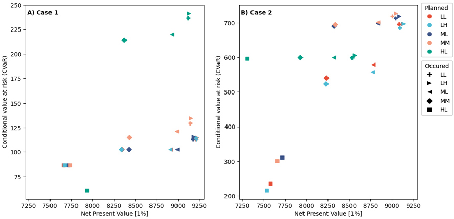
Fig. 3. A scatter plot of the two objectives (expected net present value (E(NPV)) (x-axis) and the minimum conditional value at risk (CvaR)) values across all 6 periods. Panel A) represents the cases when Equation 1A (maximizes E(NPV)) is the objective function, Panel B) represents the case when Equation 1B (minimizes the maximum CVaR). The colors represent the wind scenario assumption made when planning, while the marker represents the possible occurrence of a specific wind risk scenario. Note different scale on y-axes. View larger in new window/tab.
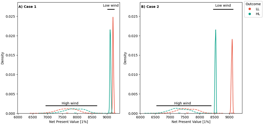
Fig. 4. The performance of the expected net present value (E(NPV)) for both cases. Case 1: is when we aim to maximize the E(NPV), while case 2 we aim to minimize the maximum conditional value at risk (CVaR). The solid lines represent the case when low intensity low frequency (LL) wind scenarios occur, while the dashed lines represent the case when high intensity low frequency (HL) wind scenarios occur. The red lines (LL) represent that planning is based on the assumption for the LL wind scenarios occur, while the green (HL) lines represent that planning is based on the assumption is the HL wind scenarios occur. View larger in new window/tab.
| Table 3. Comparison of the optimized solutions, either maximizing expected net present value (E(NPV)) or minimizing the conditional value at risk (CVaR). The payoff table describes the specific cases depending on which wind patterns are planned for versus if a different wind pattern would occur, where LL stands for low intensity low frequency wind and HL – high intensity low frequency wind. | ||||||
| MAX E(NPV) | MIN CVAR | |||||
| LL Occurs | HL Occurs | LL Occurs | HL Occurs | |||
| E(NPV) | Planned for LL | 9214 | 7657 | 9087 | 7578 | |
| Planned for HL | 9119 | 7933 | 8 535 | 7304 | ||
| CVAR | Planned for LL | Period 1 | 1774 | 1703 | 1218 | 1211 |
| Period 2 | 677 | 486 | 697 | 494 | ||
| Period 3 | 410 | 216 | 699 | 446 | ||
| Period 4 | 113 | 87 | 696 | 338 | ||
| Period 5 | 443 | 214 | 698 | 435 | ||
| Period 6 | 462 | 130 | 699 | 235 | ||
| CVAR | Planned for HL | Period 1 | 1944 | 1853 | 599 | 599 |
| Period 2 | 808 | 577 | 995 | 599 | ||
| Period 3 | 279 | 219 | 994 | 620 | ||
| Period 4 | 237 | 122 | 809 | 613 | ||
| Period 5 | 590 | 271 | 953 | 610 | ||
| Period 6 | 297 | 61 | 1018 | 597 | ||
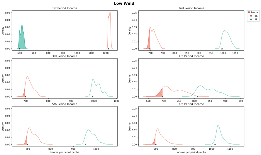
Fig. 5. The period incomes for the case when minimizing the maximum conditional value at risk (CVaR) (Case 2) when low intensity low frequency wind scenarios occur (LL). The solid red lines present the periodic incomes when planning for the low intensity low frequency (LL) wind scenarios (correct assumption). The solid green (HL) lines present the periodic incomes when planning for the high intensity low frequency wind scenarios. The shaded area of the graph indicates when the targeted income value has not been met, with the symbol at the x-axis corresponds to the CVaR value. View larger in new window/tab.
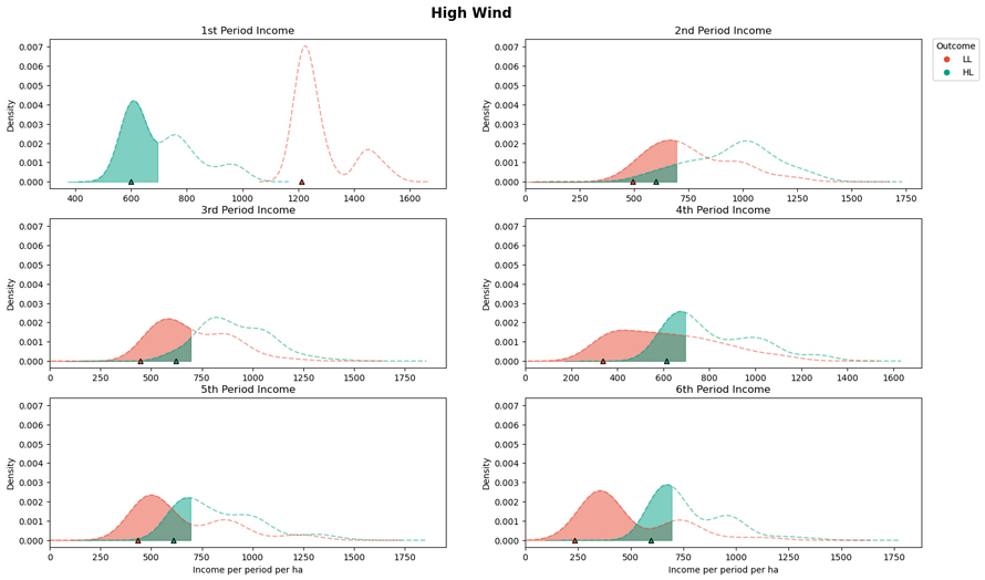
Fig. 6. The period incomes for the case when minimizing the maximum conditional value at risk (CVaR) (Case 2) when high intensity low frequency wind scenarios occur (HL). The dotted red lines (LL) present the periodic incomes when planning for the low frequency low intensity (LL) wind scenarios. The dotted green (HL) lines present the periodic incomes when planning for the high intensity low frequency wind scenarios (correct assumption). The shaded area of the graph indicates when the targeted income value has not been met, with the symbol at the x-axis corresponds to the CVaR value. View larger in new window/tab.