| Table 1. Forest attributes at plot level across the three study sites in Finland. | ||||
| Site | Suonenjoki | Hyytiälä | Liperi | |
| n | 20 | 86 | 20 | |
| Coordinates of the centres | 62°40´N, 27°07´E | 61°50´N, 24°17´E | 62°29´N, 29°05´E | |
| LAI | min. | 0.10 | 0.25 | 0.15 |
| mean | 1.99 | 2.23 | 2.04 | |
| max. | 3.71 | 4.17 | 4.19 | |
| sd | 0.90 | 0.85 | 1.04 | |
| Dominant height (m) | min. | 4.0 | 2.2 | 4.2 |
| mean | 15.7 | 16.8 | 16.2 | |
| max. | 26.9 | 34.3 | 32.6 | |
| sd | 6.5 | 6.8 | 7.0 | |
| Basal area (m2 ha–1) | min. | 4.0 | 0.5 | 1.0 |
| mean | 18.1 | 23.1 | 18.1 | |
| max. | 34.0 | 51.3 | 44.0 | |
| sd | 8.3 | 10.6 | 11.2 | |
| Abbreviations: LAI (leaf area index), min (minimum), max (maximum), sd (standard deviation). | ||||
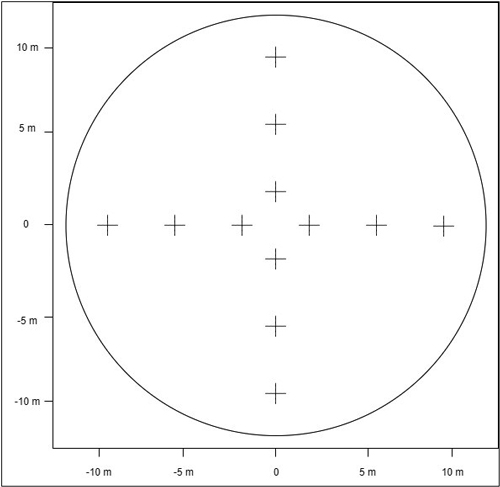
Fig. 1. Twelve measurement locations where digital hemispherical photographs (DHPs) were taken to estimate leaf area index within each r = 12.5 m plot.
| Table 2. Simulation scenarios of the number of digital hemispherical photographs to estimate leaf area index. | ||||||||||||||||||
| Scenario ID | 1 | 2 | 3 | 4 | 5 | 6 | 7 | 8 | 9 | 10 | 11 | 12 | 13 | 14 | 15 | 16 | 17 | 18 |
| No. location | 1 | 1 | 1 | 1 | 2 | 4 | 2 | 4 | 5 | 10 | 6 | 3 | 7 | 8 | 4 | 6 | 9 | 5 |
| No. images per location | 1 | 2 | 3 | 4* | 2 | 1 | 4* | 2 | 2 | 1 | 2 | 4* | 2 | 2 | 4* | 3 | 2 | 4* |
| Total No. images | 1 | 2 | 3 | 4 | 4 | 4 | 8 | 8 | 10 | 10 | 12 | 12 | 14 | 16 | 16 | 18 | 18 | 20 |
| Scenario details featured different locations where canopy images were simulated per location. Thus, the total number of images (Total No. images) equals the number of locations (No. location) multiplied by the number of images per location (No. images per location). * With four images simulated at 90° azimuth intervals per location. | ||||||||||||||||||
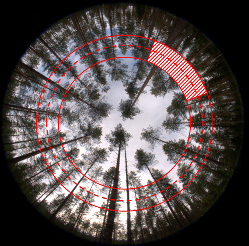
Fig. 2. Hemispherical photograph with the dash line marks the hinge angle (θ = 57°) and the mask covered 60° azimuth and ± 7.5° around the hinge angle was used to simulate smartphone canopy images.
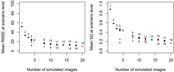
Fig. 3. Non-linear relationship between the numbers of simulated smartphone canopy images and their ![]() (left) and
(left) and ![]() (right) at scenario level. The labels represented Scenario IDs and red colour denoted scenarios where images were simulated at 90° azimuth intervals. Scenario 18 was selected for further inspection.
(right) at scenario level. The labels represented Scenario IDs and red colour denoted scenarios where images were simulated at 90° azimuth intervals. Scenario 18 was selected for further inspection.
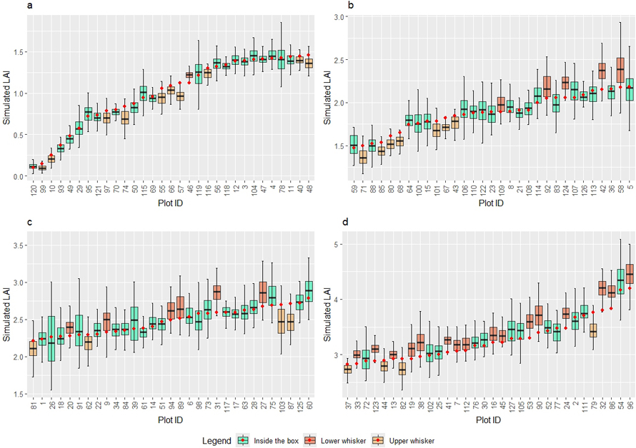
Fig. 4. Boxplots illustrating the simulated leaf area index and their observed counterparts (red dot) at plots based on their leaf area index quantiles: Q1 (a), Q2 (b), Q3 (b) and Q4 (d). View larger in new window/tab.
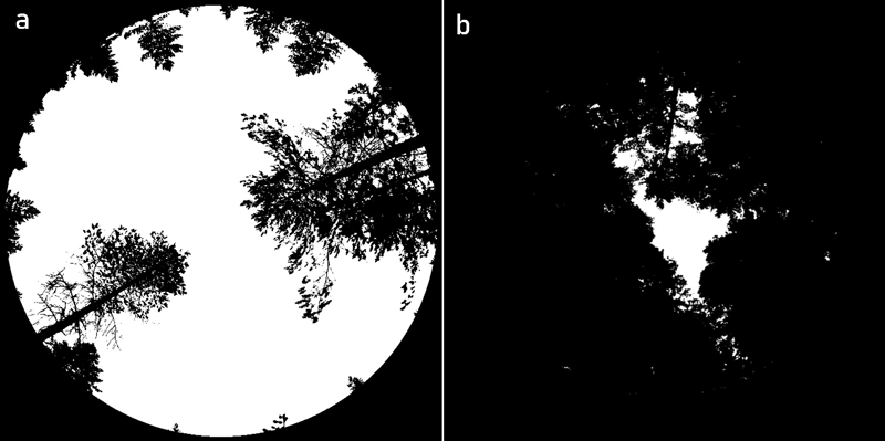
Fig. 5. Binary digital hemispherical photographs where gap fraction was influenced by seed trees in seedling stand (a) and by small random big gaps on a dense canopy stand (b).
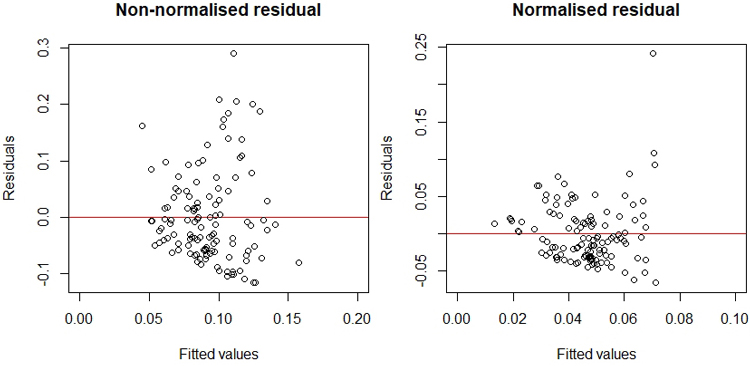
Fig. 6. Residual analysis with the scatter plots of the non-normalised mean absolute model residuals ![]() (left) and the normalised mean absolute model residuals
(left) and the normalised mean absolute model residuals ![]() (right) with fitted values.
(right) with fitted values.
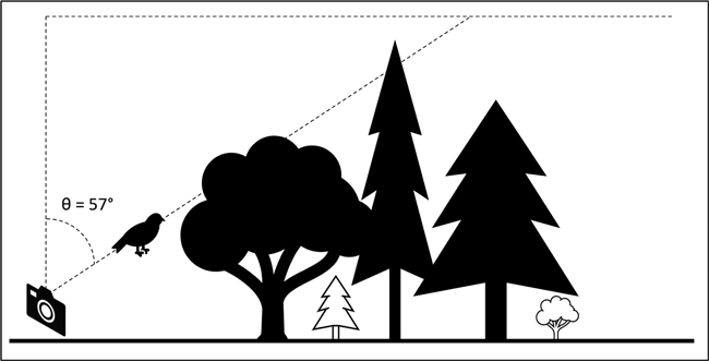
Fig. 7. Illustration of citizen scientists taking images at the hinge angle (θ = 57°) following gamified instructions. A bird will appear on the screen of the smartphone screen to help participants to locate the angle and capture images.