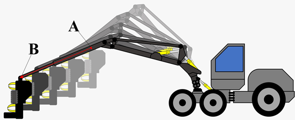
Fig. 1. Simplified illustration of the general principle of boom-tip control. The red arrow indicates the boom-tip’s optimal path (typically the shortest) from its initial (A) to final (B) position. Conducting even such a seemingly simple crane manoeuvre requires precisely controlling different crane parts to combine them into the desired boom-tip path. When using boom-tip control, operators steer the boom-tip directly rather than controlling separate crane parts (i.e. booms and extension). The illustration is based on a generic harvester-crane construction sketch by Gerasimov and Siounev (1998).
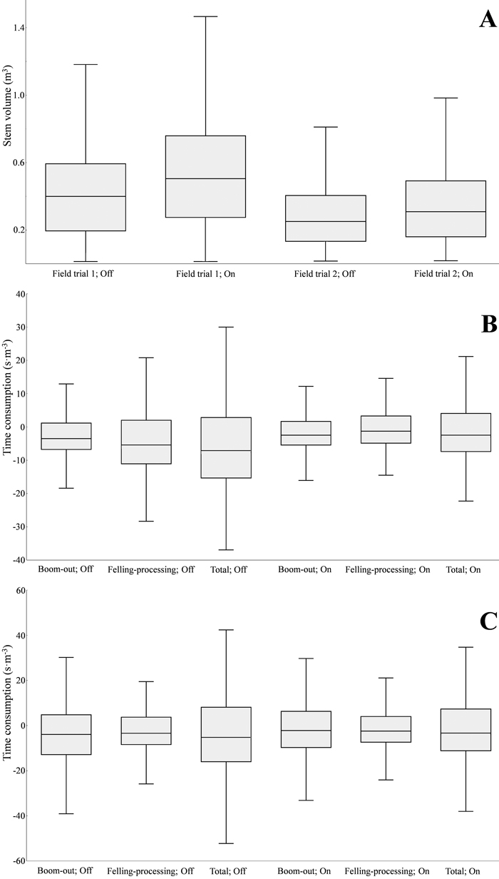
Fig. 2. Stem-volume distributions per plot (A), described using interquartile ranges (IQRs). The label “On” denotes IBC activated, and “Off” denotes IBC deactivated. Residual distributions for time-consumption models – both total and work-element-specific – are described using IQRs for field trial 1 (B) and field trial 2 (C). In all panels (A, B, and C), the IQRs are supplemented with whiskers according to Tukey’s 1.5·IQR rule.
| Table 1. Mean squares, F-values, and p-values from the analysis of covariance (ANCOVA) for effective time consumption (seconds per solid m3 under bark), presented either as a total or divided into work elements. Stem volume–1 is the covariate, the boom-control system, i.e. IBC (levels: off and on) and tree species (levels: spruce, pine and birch) are the categorical factors. The unit of observation is a tree (i.e. stem). The total number of trees in field trial 1 was 928, and in field trial 2, it was 1024. | |||||
| Dependent variable | Effect | Field trial | Mean square | F-value | P-value |
| Total time | Intercept | 1 | 64498.94 | 11.13 | 0.0009 |
| 2 | 48022.00 | 18.41 | <0.0001 | ||
| Stem volume–1 | 1 | 12734908.90 | 2197.24 | <0.0001 | |
| 2 | 15117065.02 | 5794.65 | <0.0001 | ||
| IBC | 1 | 22697.41 | 3.92 | 0.0481 | |
| 2 | 209.83 | 0.08 | 0.7768 | ||
| Tree species | 1 | 444.72 | 0.08 | 0.9261 | |
| 2 | 4969.56 | 1.90 | 0.1494 | ||
| Boom-out | Intercept | 1 | 1225.05 | 1.20 | 0.2741 |
| 2 | 739.95 | 0.40 | 0.5297 | ||
| Stem volume–1 | 1 | 1652909.06 | 1615.63 | <0.0001 | |
| 2 | 3064558.05 | 1636.62 | <0.0001 | ||
| IBC | 1 | 264.94 | 0.26 | 0.6110 | |
| 2 | 151.42 | 0.08 | 0.7762 | ||
| Tree species | 1 | 1.02 | 0.00 | 0.9990 | |
| 2 | 2759.61 | 1.47 | 0.2295 | ||
| Felling-processing | Intercept | 1 | 47946.00 | 10.40 | 0.0013 |
| 2 | 36839.87 | 43.36 | <0.0001 | ||
| Stem volume–1 | 1 | 5211839.25 | 1130.14 | <0.0001 | |
| 2 | 4568816.85 | 5377.88 | <0.0001 | ||
| IBC | 1 | 18057.85 | 3.92 | 0.0481 | |
| 2 | 4.75 | 0.01 | 0.9404 | ||
| Tree species | 1 | 418.43 | 0.09 | 0.9133 | |
| 2 | 392.30 | 0.46 | 0.6303 | ||
| Because the factor tree species did not statistically significantly contribute to the ANCOVA models or improve residual behaviour, it was removed from the final time-consumption models used in the post-hoc analysis (Table 2). The final time-consumption models are available in Supplementary file S1. | |||||
| Table 2. Least squares means (LSMs) for effective time consumption (seconds per solid m3 under bark) obtained from the ANCOVA (Table 1). LSMs are followed by the lower and the upper confidence limits (LCL; UCL) of the 95% confidence interval, and the number of trees (n). Statistically significant time savings with activated IBC are given in percentages (p < 0.05, Tukey-Kramer method). A hyphen “-” indicates the lack of a statistically significant difference between the boom-control systems (i.e. IBC: off/on). | ||||||||||
| Field trial | Dependent variable | IBC: off (s m–3) | IBC: on (s m–3) | Time saving | ||||||
| LSM | LCL | UCL | n | LSM | LCL | UCL | n | |||
| 1(a | Total time | 99.3 | 92.1 | 106.4 | 440 | 89.3 | 82.5 | 96.1 | 488 | 10.1% |
| Boom-out | 27.9 | 24.9 | 30.9 | 26.8 | 23.9 | 29.6 | - | |||
| Felling-processing | 71.4 | 65.0 | 77.8 | 62.5 | 56.4 | 68.5 | 12.5% | |||
| 2(b | Total time | 118.7 | 113.8 | 123.7 | 418 | 119.4 | 115.4 | 123.5 | 606 | - |
| Boom-out | 42.2 | 38.1 | 46.4 | 42.9 | 39.4 | 46.3 | - | |||
| Felling-processing | 76.5 | 73.7 | 79.3 | 76.6 | 74.2 | 78.9 | - | |||
| a) LSMs at stem volume–1 = 4.877 b) LSMs at stem volume–1 = 6.864 | ||||||||||