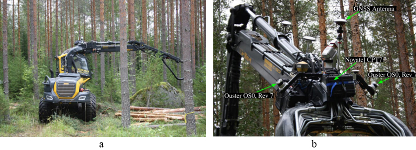
Fig. 1. Study site and the Ponsse Scorpion harvester used for the study (a), and the position of the two Ouster LiDARs, one GNSS antenna, and Novatel CPT7 installed on the boom of the Ponsse harvester (b). The Novatel CPT7 was behind the black box attached to the aluminium frame, not inside the black box.
| Table 1. Technical specifications of the LiDAR systems used in this study. | |||
| LiDAR system | Lasers wavelength (nm) | Beam radius at exit (mm) | Divergence (mrad) |
| Riegl VUX-1HA | 1550 | 4.5 | 0.5 |
| Riegl VUX-120 | 1550 | NA | 0.4 |
| GeoSLAM Zeb Horizon RT | 903 | 12.7 (horizontal) × 9.5 (vertical) | 3.0 × 1.2, 300 kHz |
| Ouster OS0 (Rev 7) | 865 | 5 | 6 |
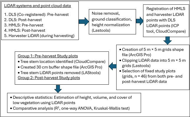
Fig. 2. Workflow for the plot level analysis and comparing consistencies among HMLS, DLS and harvester LiDAR points for low vegetation quantification in this study.
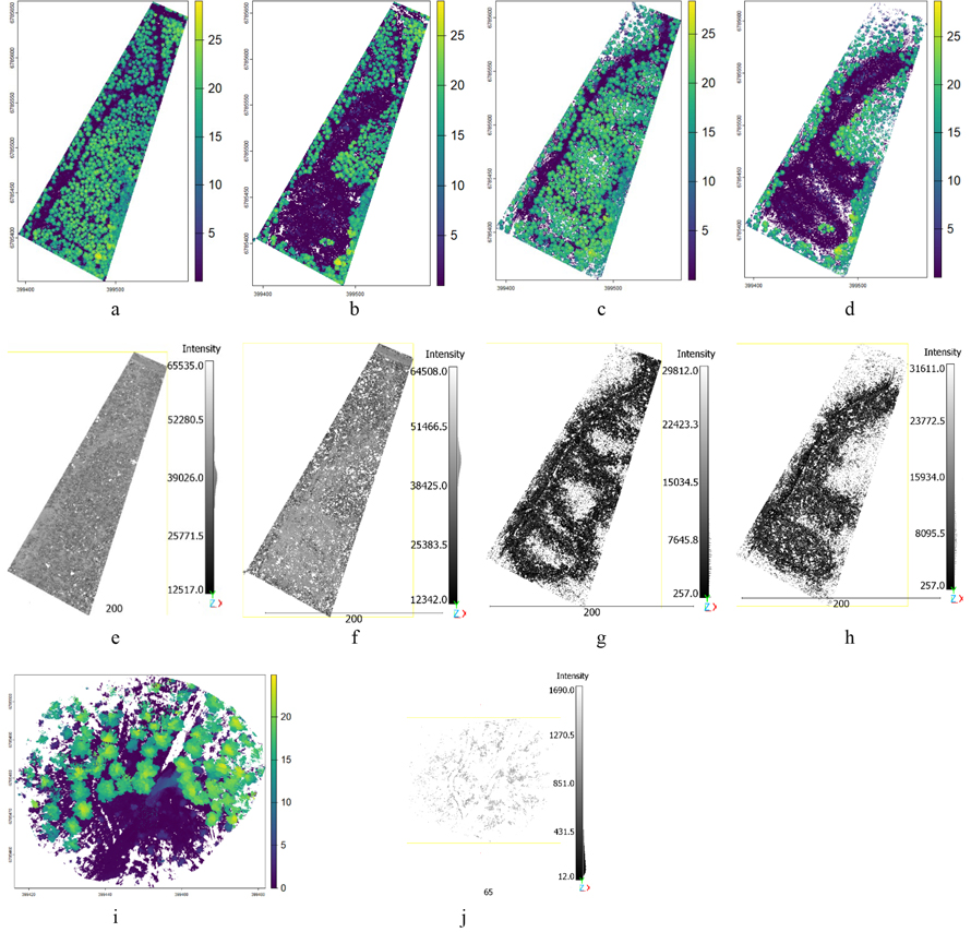
Fig. 3. LiDAR point clouds showing vegetation points (a–d, i) by canopy height and ground points (e–h, j) by intensity values: DLS preharvest (a, e), DLS postharvest (b, f), HMLS preharvest (c, g), HMLS postharvest (d, h), and harvester LiDAR (i, j). View larger in new window/tab.
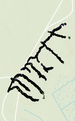
Fig. 4. Harvester trajectory. During the harvesting operations, the trajectory of the harvester was monitored using a robotic total station.
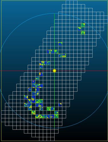
Fig. 5. Harvested area divided into 5 m × 5 m plots (grid cells) and selected plots for study containing point clouds (DLS post-harvest LiDAR point clouds).
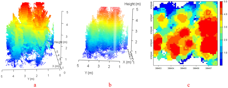
Fig. 6. Visualization of low vegetation structure: Point clouds (a), 10 cm voxels (b), and canopy height with grid size 10 cm (c) (Plot code: Plot 102: harvester LiDAR before harvesting operations).
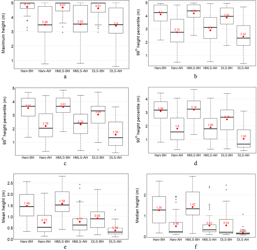
Fig. 7. Low vegetation height metrics (in meters) derived from three LiDAR systems (harvester LiDAR (Harv), HMLS, and DLS) before harvest (BH) and after harvest (AH): (a) maximum height, (b) 99th height percentile, (c) 95th height percentile, (d) 90th height percentile, (e) mean height, and (f) median height. Red points and red numerical values indicate the mean values.
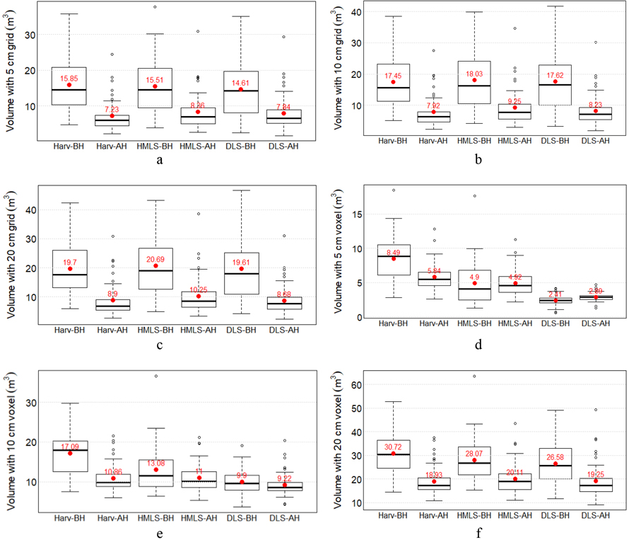
Fig. 8. Low vegetation points-occupied volume metrics (m3 per plot of 25 m2) from three LiDAR systems before and after harvesting. Volumes were estimated using the mean height method with 5 cm (a), 10 cm (b), and 20 cm (c) grids, and by fitting voxels of 5 cm (d), 10 cm (e), and 20 cm (f).
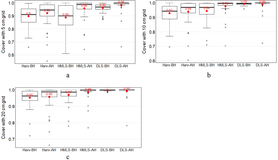
Fig. 9. Low vegetation cover metrics from three LiDAR systems before and after harvesting. Cover was estimated using 5 cm (a), 10 cm (b), and 20 cm grids (c).
| Table 2. Results of ANOVA and Kruskal–Wallis test on harvester, HMLS and DLS LiDAR for quantifying low vegetation attributes. Test values for one way ANOVA is F-statistic value (F) and for Kruskal–Wallis test Chi-square value (χ2). Short form written in the Test columns: K–W indicate Kruskal–Wallis test, ANOVA indicate one-way ANOVA, and logt, Sqrt, and Box-Cox represent the data transfomation process used to proceeed with one-way ANOVA test. p-values in bold indicate statistical significance (p < 0.05). | ||||||||||||
| Low vegetation attributes | Pre-harvest | Post-harvest | ||||||||||
| Test value | p-value | Adjusted p-value | Test | Test value | p-value | Adjusted p-value | Test | |||||
| Harvester – DLS | HMLS – DLS | HMLS – Harvester | Harvester – DLS | HMLS – DLS | HMLS – Harvester | |||||||
| Maximum height (m) | 0.682 | 0.718 | 0.632 | 0.853 | 1.000 | K–W | 0.405 | 0.820 | 1.000 | 0.796 | 1.000 | K–W |
| 99th height percentile (m) | 3.809 | 0.149 | 0.320 | 0.081 | 0.744 | K–W | 4.863 | 0.087 | 0.198 | 0.047 | 0.779 | K–W |
| 95th height percentile (m) | 8.948 | 0.011 | 0.037 | 0.006 | 0.825 | K–W | 11.870 | 0.0026 | 0.0096 | 0.0021 | 0.960 | K–W |
| 90th height percentile (m) | 8.138 | 0.0004 | 0.004 | 0.0008 | 0.855 | ANOVA | 18.570 | 9.25e-05 | 0.0005 | 0.0002 | 1.000 | K–W |
| Mean height (m) | 19.75 | 3.01e-08 | 0.0000 | 0.0000 | 0.716 | Box-Cox | 21.810 | 1.83e-05 | 0.0004 | 0.0000 | 0.771 | K–W |
| Median height (m) | 39.092 | 3.24e-09 | 0.0000 | 0.0000 | 0.669 | K–W | 40.517 | 1.59e-09 | 0.0000 | 0.0000 | 0.250 | K–W |
| Volume with 5 cm grid (m3) | 0.721 | 0.488 | 0.500 | 0.624 | 0.978 | Sqrt | 0.984 | 0.377 | 0.816 | 0.708 | 0.344 | logt |
| Volume with 10 cm grid (m3) | 0.058 | 0.943 | 0.999 | 0.948 | 0.958 | Sqrt | 1.343 | 0.264 | 0.951 | 0.428 | 0.273 | Box-Cox |
| Volume with 20 cm grid (m3) | 0.209 | 0.812 | 0.959 | 0.795 | 0.927 | logt | 1.611 | 0.204 | 0.980 | 0.232 | 0.317 | Box-Cox |
| Volume with 5 cm voxel (m3) | 75.229 | 2.2e-16 | 0.0000 | 0.0001 | 0.0000 | K–W | 66.027 | 4.59e-15 | 0.0000 | 0.0000 | 0.058 | K–W |
| Volume with 10 cm voxel (m3) | 38.793 | 3.76e-09 | 0.0000 | 0.0132 | 0.0005 | K–W | 4.618 | 0.0115 | 0.036 | 0.018 | 0.966 | Box-Cox |
| Volume with 20 cm voxel (m3) | 2.674 | 0.072 | 0.059 | 0.613 | 0.366 | logt | 0.755 | 0.472 | 0.993 | 0.507 | 0.573 | Box-Cox |
| Cover with 5 cm grid | 18.511 | 9.55e-05 | 0.0001 | 0.0010 | 0.846 | K–W | 42.358 | 6.33e-10 | 0.0000 | 0.0003 | 0.0085 | K–W |
| Cover with 10 cm grid | 47.828 | 4.11e-11 | 0.0000 | 0.0000 | 0.079 | K–W | 48.547 | 2.87e-11 | 0.0000 | 0.0021 | 0.0003 | K–W |
| Cover with 20 cm grid | 48.470 | 2.97e-11 | 0.0000 | 0.0000 | 0.025 | K–W | 42.812 | 5.05e-10 | 0.0000 | 0.082 | 0.0000 | K–W |