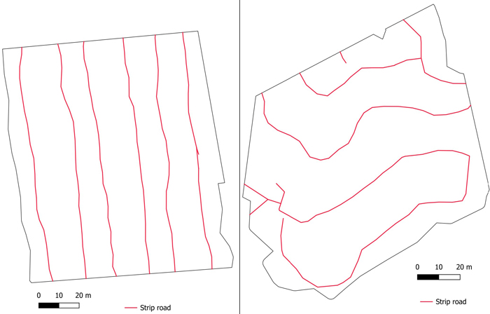
Fig. 1. On the left, an example of a straightforward and on the right, an example of a curvy strip road network on the measurement area.
| Table 1. Stand variables from the measurement areas. These include the total length of the strip road per hectare after thinning, main tree species, and shape description of the strip road network. | |||||
| Measurement area ID | Area, ha | Municipality | Strip road density, m ha–1 | Main tree species | Strip road network shape |
| A | 0.7 | Teuva | 589 | Spruce | Curvy |
| B | 1.2 | Sastamala | 610 | Pine | Straightforward |
| C | 1.0 | Sastamala | 522 | Pine | Curvy |
| D | 1.0 | Teuva | 533 | Pine | Straightforward |
| E | 0.9 | Sastamala | 488 | Pine | Curvy |
| F | 1.2 | Teuva | 436 | Pine | Straightforward |
| G | 0.8 | Teuva | 536 | Pine | Straightforward |
| Mean | 1.0 | 531 | |||
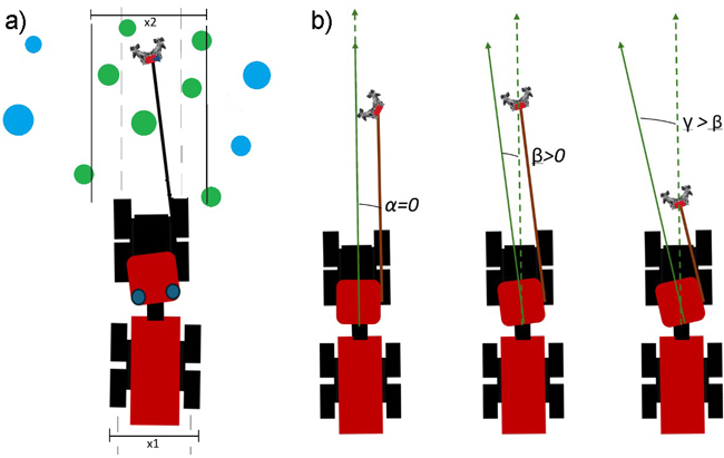
Fig. 2. a) Illustration showing identification of the strip road trees. Here, x1 is the width of the harvester (2.8 m) and x2 is the width of the strip road zone (3.2 m). b) Illustration showing how asymmetry in the Komatsu harvester affects the boom angle. The angles α, β and γ show the angle between the boom and the middle line of the harvester’s front frame and demonstrate how this angle changes when the harvester’s head is moved in relation to the middle line of the harvester.

Fig. 3. Distance distribution of all harvested stems, showing the distance from the middle line of the harvester. Substantially higher frequency close to the middle line of the harvester demonstrates our method to identify strip road trees.

Fig. 4. The workflow of the estimation method outlines the calculation steps of diameter distributions and to estimate hectare-wise growing stock after thinning.
| Table 2. Description of measurement areas before first thinning. The table contains measurement areas, their strip road densities and the numerically estimated stem counts and basal areas based on our method. In addition, reference values are shown, as well as their relative differences. | ||||||
| Measurement area ID | Estimated stem count, N ha–1 | Reference stem count, N ha–1 | Diff-% | Estimated basal area, m2 ha–1 | Reference basal area, m2 ha–1 | Diff-% |
| A | 1596 | 1641 | –2.7 | 22.0 | 24.4 | –10.0 |
| B | 1369 | 1203 | 13.8 | 17.4 | 16.2 | 7.5 |
| C | 1749 | 1671 | 4.7 | 24.1 | 24.9 | –3.2 |
| D | 1586 | 1602 | –1.0 | 22.0 | 24.4 | –9.6 |
| E | 1399 | 1376 | 1.7 | 22.4 | 24.1 | –7.0 |
| F | 1500 | 1363 | 10.1 | 22.2 | 22.0 | 0.9 |
| G | 2016 | 1771 | 13.8 | 27.1 | 26.6 | 1.7 |
| Mean | 1602 | 1518 | 5.5 | 22.5 | 23.2 | –3.3 |
| Table 3. Description of numerical results of measurement areas after first thinning. Estimated stem counts, basal areas based on our method presented earlier in this paper. In addition, reference values, and their relative differences are shown. | ||||||
| Measurement area ID | Estimated stem count, N ha–1 | Reference stem count, N ha–1 | Diff-% | Estimated basal area, m2 ha–1 | Reference basal area, m2 ha–1 | Diff-% |
| A | 770 | 1016 | –24.2 | 12.6 | 17.8 | –29.1 |
| B | 720 | 552 | 30.4 | 10.3 | 9.1 | 13.1 |
| C | 860 | 797 | 7.9 | 13.4 | 14.4 | –7.0 |
| D | 729 | 809 | –9.9 | 12.8 | 16.0 | –21.9 |
| E | 758 | 841 | –9.9 | 13.4 | 16.7 | –19.9 |
| F | 859 | 733 | 17.2 | 14.5 | 14.4 | 1.0 |
| G | 1103 | 1023 | 7.8 | 16.5 | 19.4 | –15.0 |
| Mean | 828 | 824 | 0.5 | 13.3 | 15.4 | –13.6 |
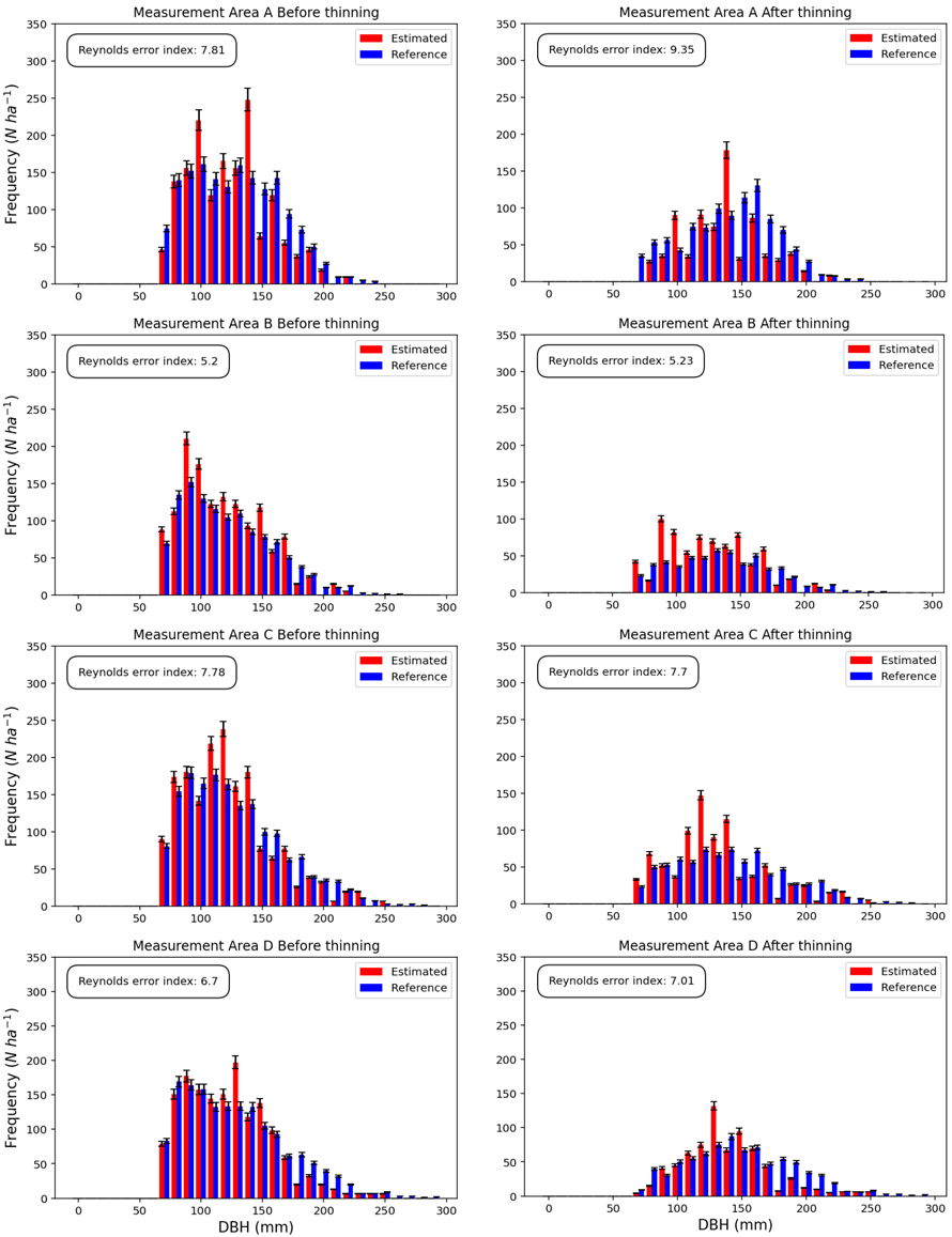
Fig. 5a. Illustration of estimated and reference diameter distributions with uncertainties before and after thinning of measurement areas A–D. Reynold’s error index and visual interpretation indicates that estimated and reference distributions differ only a little. Abbreviation DBH means diameter at breast height.

Fig. 5b. Illustration of estimated and reference diameter distributions with uncertainties before and after thinning of measurement areas E–G. Reynold’s error index and visual interpretation indicates that estimated and reference distributions differ only a little. Abbreviation DBH means diameter at breast height.