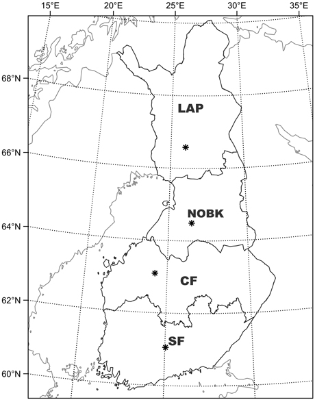
Fig. 1. Stand characteristics and weather data in the simulations represented conditions in Southern Finland (SF), Central Finland (CF), Northern Ostrobothnia–Kainuu (NOBK) and Lapland (LAP).
| Table 1. Locations and coordinates of the weather stations in Southern Finland (SF), Central Finland (CF), Northern Ostrobothnia–Kainuu (NOBK) and Lapland (LAP) and mean annual temperature sum and precipitation in the studied regions, and the precipitation in exceptionally dry years of 2006 and 2018. | ||||||
| Main region | Weather data location | Longitude | Latitude | Mean annual temperature sum (dd) | Mean annual precipitation (mm) | Precipitation 2006 / 2018 (mm) |
| SF | Hämeenlinna | 25.04°E | 61.05°N | 1412 | 635 | 587 / 434 |
| CF | Alajärvi | 24.26°E | 63.09°N | 1214 | 640 | 508 / 427 |
| NOBK | Vaala | 26.47°E | 64.49°N | 1156 | 649 | 613 / 471 |
| LAP | Rovaniemi | 26.01°E | 66.58°N | 1035 | 552 | 408 / 472 |
| Table 2. Drained peatland site types, fertility class descriptions, fertility classes (Vasander and Laine 2008), peat types and main tree species. Fertility class describes site fertility in ascending order where 2 is the most nutrient rich and 5 is the most nutrient poor. | ||||
| Drained peatland site type | Fertility class description | Fertility class | Peat type | Main tree species |
| Herb-rich | Fertile | 2 | Carex | Norway spruce |
| Bilberry (Vaccinium myrtillus L.) | Medium-fertile | 3 | Carex | Norway spruce or Scots pine |
| Lingonberry (Vaccinium vitis-idaea L.) | Medium-poor | 4 | Carex | Scots pine |
| Dwarf shrub | Poor | 5 | Sphagnum | Scots pine |
| Table 3. Forest input data for the simulations. The fertility class according to Table 2 are: 2 is fertile, 3 is medium-fertile, 4 is medium-poor and 5 is poor. Main tree species are: 1 is Scots pine (Pinus sylvestris L.) and 2 is Norway spruce (Picea abies (L.) Karst.). Abbreviations for the forest attributes are: stem number (Ns), basal area (BA), basal area-weighted mean diameter (Dg), basal area-weighted mean height (Hg), dominant height (Hdom) and stand volume (Vol). Regions codes are: SF is Southern Finland, CF is Central Finland, NOBK is Northern Ostrobothnia–Kainuu and LAP is Lapland. | ||||||||
| Region | Fertility class | Main species | Ns (ha–1) | BA (m2 ha–1) | Dg (cm) | Hg (m) | Hdom (m) | Vol (m3 ha–1) |
| SF | 2 | 2 | 1070 | 22.6 | 20.3 | 16.4 | 19.2 | 178 |
| SF | 3 | 2 | 850 | 20.2 | 21.3 | 17.4 | 19.7 | 169 |
| SF | 3 | 1 | 930 | 19.8 | 22 | 17.9 | 20.2 | 168 |
| SF | 4 | 1 | 920 | 16.8 | 20.2 | 16.6 | 18.6 | 134 |
| SF | 5 | 1 | 1160 | 15.1 | 15 | 12.3 | 14.4 | 94 |
| CF | 2 | 2 | 900 | 21.1 | 21.8 | 15.3 | 17.9 | 149 |
| CF | 3 | 2 | 1110 | 19.2 | 18.9 | 15.6 | 18.4 | 144 |
| CF | 3 | 1 | 1390 | 20.5 | 17.3 | 14.7 | 17.4 | 147 |
| CF | 4 | 1 | 870 | 16.1 | 18.9 | 15.6 | 17.7 | 122 |
| CF | 5 | 1 | 1020 | 13.6 | 15.7 | 12.2 | 14.3 | 84 |
| NOBK | 2 | 2 | 1420 | 20 | 18.1 | 12.7 | 15.4 | 120 |
| NOBK | 3 | 2 | 1330 | 19.1 | 17.9 | 14.1 | 17 | 130 |
| NOBK | 3 | 1 | 1300 | 19 | 17.2 | 14.1 | 16.4 | 132 |
| NOBK | 4 | 1 | 1130 | 16 | 16.4 | 13.3 | 15.5 | 106 |
| NOBK | 5 | 1 | 1270 | 12.9 | 13.9 | 10.8 | 12.8 | 71 |
| LAP | 2 | 2 | 1640 | 20.6 | 16.5 | 11.4 | 13.8 | 113 |
| LAP | 3 | 2 | 1820 | 19.3 | 16.2 | 12.7 | 15.6 | 118 |
| LAP | 3 | 1 | 1900 | 20.2 | 14.6 | 11.6 | 14 | 119 |
| LAP | 4 | 1 | 2220 | 16.4 | 12.3 | 9.5 | 12.3 | 81 |
| LAP | 5 | 1 | 2080 | 12.4 | 10.6 | 8.2 | 10.2 | 55 |
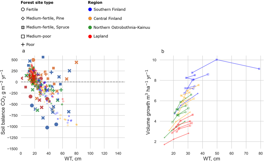
Fig. 2. a) Dependence of annual soil CO2 balance on the growing season water table (WT) in SUSI simulations (small, slightly transparent markers) and in experimental data presented by Ojanen and Minkkinen (2019) (large markers). Positive y-values indicate a C sink and negative C source. b) Dependence of mean stand volume growth (current annual increment) on the mean WT during the growing season. Each site was simulated with 0.3 m, 0.6 m and 0.9 m ditch depths resulting in different growing season WTs. Marker colours indicate geographical location (Fig. 1) and marker style different site fertility classes (Table 3). Mtkg sites include both Scots pine and Norway spruce stands in a and b.
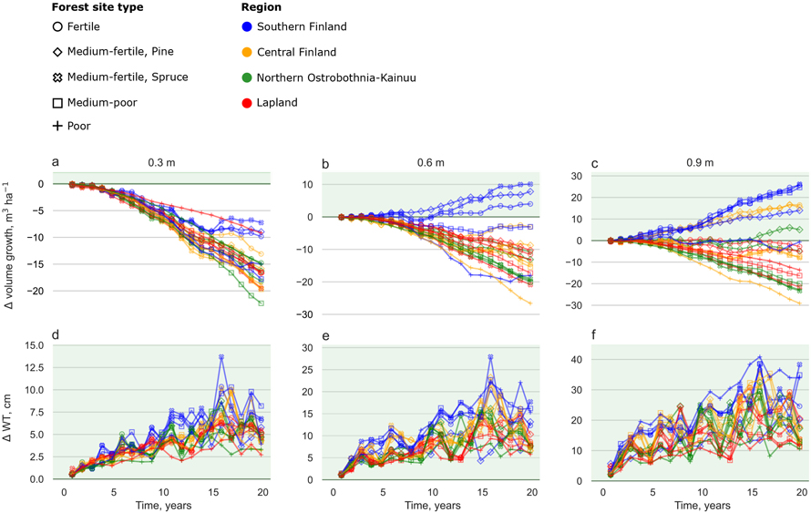
Fig. 3. Cumulative difference between the ditch shallowing and reference scenarios for volume growth (a–c) during a 20-year period and annual difference in water table (WT) (d–f) in different site types and regions. Each site was simulated with 0.3 m (leftmost column), 0.6 m (centre column) and 0.9 m (rightmost column) initial ditch depths. Marker colours indicate geographical location (Fig. 1) and marker style different site fertility classes (Table 3). Note different scales in the y-axis between different ditch depth scenarios. Years 3 and 15 were dry and warm years 2006 and 2018, respectively. View larger in new window/tab.
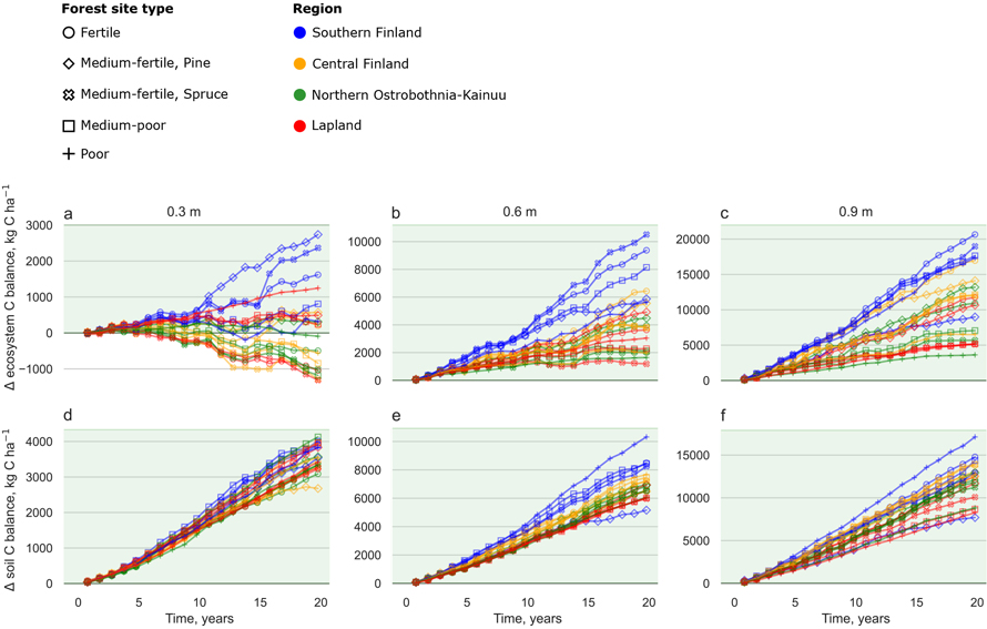
Fig. 4. Cumulative difference between the ditch shallowing and reference scenarios for ecosystem C balance (a–c) and soil C balance (d–f) during a 20-year period in different site types and regions. Each site was simulated with 0.3 m (leftmost column), 0.6 m (centre column) and 0.9 m (rightmost column) initial ditch depths. Marker colours indicate geographical location (Fig. 1) and marker style different site fertility classes (Table 3). Note different scales in the y-axis between different ditch depth scenarios. Years 3 and 15 were dry and warm years 2006 and 2018, respectively. View larger in new window/tab.
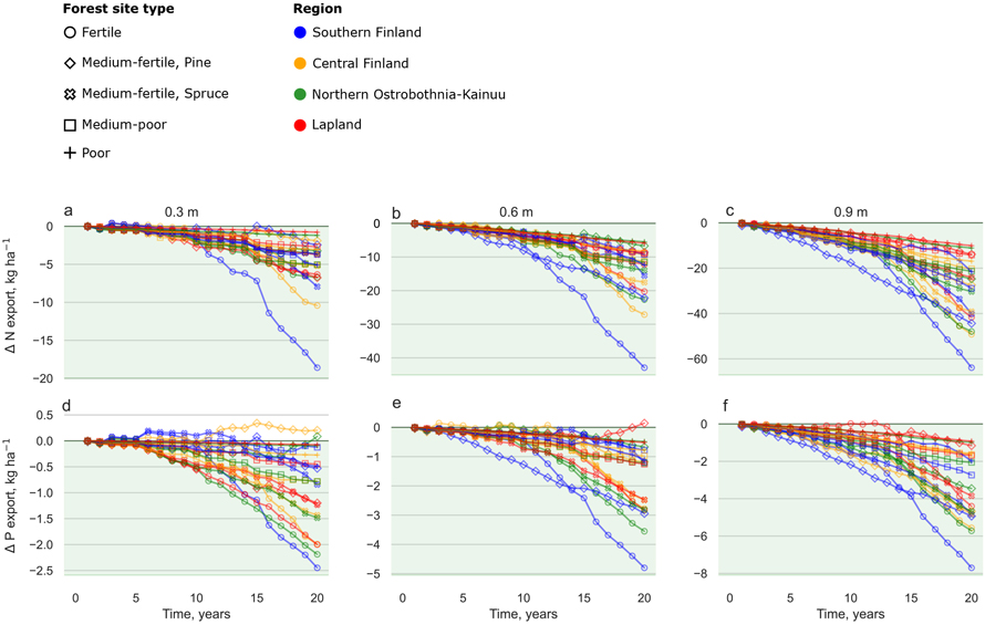
Fig. 5. Cumulative difference between the ditch shallowing and reference scenarios for N exports (a–c) and P exports (d–f) during a 20-year period in different site types and regions. Each site was simulated with 0.3 m (leftmost column), 0.6 m (centre column) and 0.9 m (rightmost column) initial ditch depths. Marker colours indicate geographical location (Fig. 1) and marker style different site fertility classes (Table 3). Note different scales in the y-axis between different ditch depth scenarios. Years 3 and 15 were dry and warm years 2006 and 2018, respectively. View larger in new window/tab.