| Table 1. Population names, their geographical locations, number of individuals sampled for genetic analyses, parameters of genetic diversities and inbreeding coefficients (F) for B. nana sampling sites studied. Ploc = number of polymorphic loci; Hj = Nei’s gene diversity. | ||||||||
| Country | Population | Code | Location | No of individuals | Ploc | Hj | F | |
| Latitude, Longitude | ||||||||
| 1. | Poland | Linje | LIN | 53°11´N, 18°18´E | 23 | 83 | 0.120 | 0.249 |
| 2. | Torfowisko pod Zieleńcem | ZIEL | 50°20´N, 16°25´E | 20 | 91 | 0.129 | 0.130 | |
| 3. | Torfowiska Doliny Izery | IZER | 50°51´N, 15°21´E | 20 | 102 | 0.136 | 0.060 | |
| 4. | Finland | Juttuvaara | JUT | 62°57´N, 30°22´E | 21 | 87 | 0.103 | 0.075 |
| 5. | Kaitaa | KAI | 63°14´N, 28°52´E | 20 | 87 | 0.114 | 0.402 | |
| 6. | Tuusniemi | TUS | 62°52´N, 28°24´E | 21 | 91 | 0.091 | 0.035 | |
| 7. | Belarus | Berezin’skij Zapovednik | BZ | 54°37´N, 28°21´E | 7 | 85 | 0.120 | 0.078 |
| 8. | Russia | Ural Mts. | UR | 63°03´N, 58°36´E | 7 | 89 | 0.115 | 0.057 |
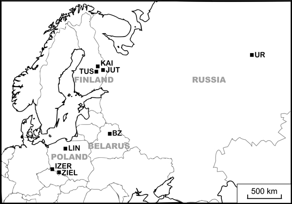
Fig. 1. Locations of study populations. Population codes according to Table 1.
| Table 2. Parameters of habitat quality and sexual reproduction in the B. nana populations. Pop = populations codes according to Table 1; Hab = number of habitat plots; Habitat quality parameters: EC = electrical conductivity; Reproductive parameters: GS = number of germinated (without scarification) seeds per individual, GSC = number of seeds germinated after scarification, ES = number of empty seeds (without ovule), PF = number of partly filled seeds, IN = number of seeds infected by insects; # = median values. View in new window/tab. |
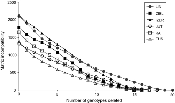
Fig. 2. The graph of matrix incompatibility counts (MICs). Reduction of MIC is related to the successive removal of genotypes from each of the specific population. Graphic symbols refer to codes of populations described in Table 1.
| Table 3. Results from analyses of molecular variance in the B. nana populations divided into two groups: LIN + ZIEL (Poland) and all other samples. | |||
| Source of variation | Percentage of variation | P | Fixation indices |
| Among groups | 12.87 | 0.032 | FCT = 0.12866 |
| Among localities within groups | 15.82 | < 0.0001 | FSC = 0.18153 |
| Within localities | 71.32 | < 0.0001 | FST = 0.28684 |
| Table 4. Genetic differentiation (FST) between pairs of populations of B. nana. Population codes according to Table 1. * = statistically significant values after Bonfferoni’ s correction. | |||||||
| ZIEL | IZER | JUT | KAI | TUS | BZ | UR | |
| LIN | 0.244* | 0.271* | 0.314* | 0.196* | 0.339* | 0.228* | 0.278* |
| ZIEL | 0.234* | 0.359* | 0.249* | 0.367* | 0.285* | 0.301* | |
| IZER | 0.246* | 0.159* | 0.252* | 0.222* | 0.261* | ||
| JUT | 0.049* | 0.051* | 0.161* | 0.203* | |||
| KAI | 0.085* | 0.097* | 0.136* | ||||
| TUS | 0.176* | 0.217* | |||||
| BZ | 0.037 | ||||||
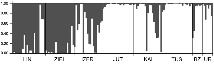
Fig. 3. Clustering results for the B. nana populations (K = 2) generated by STRUCTURE software. Population codes according to Table 1.
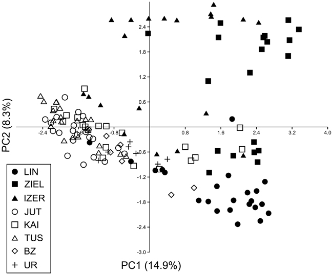
Fig. 4. Principal component analysis (PCA) plot revealing the genetic distances among 139 individuals of B. nana. Graphic symbols refer to codes of populations described in Table 1.
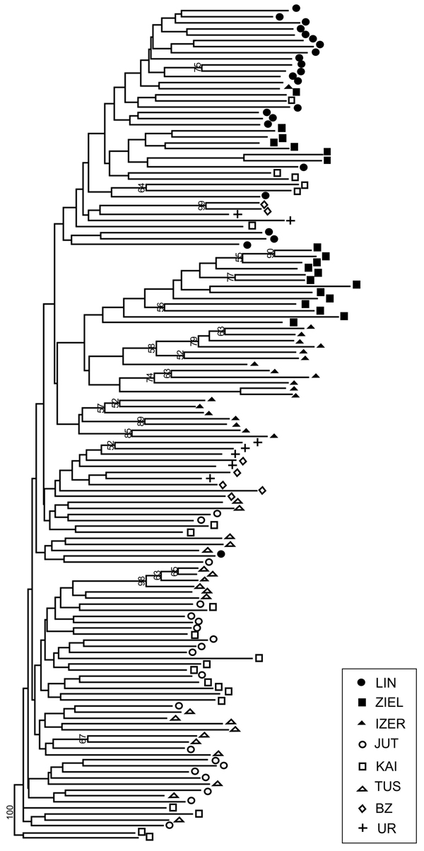
Fig. 5. Neighbour-joining tree based on 240 AFLP fragments comprising 8 populations of B. nana (based on Jaccard’s similarity coefficient; Hammer et al. 2001). Numbers on branches represent bootstrap support (1000 replicates). Graphic symbols refer to codes of populations described in Table 1.
| Table 5. Results of the two-sample randomisation tests comparing the reproductive parameters (dependent variable) in the relict (R) vs. central (C) populations (grouping variables). * = value significant after Bonferroni’s correction. | ||||
| Variable | Test statistic | P | ||
| Grouping | Dependent | Medians | ||
| Relict vs. central samples | Female flowers | R = 1.0000 | 1.0000 | 0.3956 |
| C = 0.0000 | ||||
| Male flowers | R = 6.0000 | 3.0000 | 0.0074* | |
| C = 3.0000 | ||||
| Total no. of flowers | R = 7.5000 | 3.0000 | 0.0161 | |
| C = 4.5000 | ||||
| Seed mass [g] | R = 0.0159 | 0.0027 | 0.0035* | |
| C = 0.0132 | ||||
| Seeds germinated without scarification | R = 0.0000 | 0.0000 | 1.0000 | |
| C = 0.0000 | ||||
| Seeds germinated after scarification | R = 0.5000 | –3.5000 | 0.0002* | |
| C = 4.0000 | ||||
| Empty seeds | R = 95.5000 | 0.5000 | 0.7345 | |
| C = 95.0000 | ||||
| Partly filled seeds | R = 0.0000 | 0.0000 | 1.0000 | |
| C = 0.0000 | ||||
| Seeds infected by insects | R = 1.0000 | 0.0000 | 1.0000 | |
| C = 1.0000 | ||||
| Table 6. Results of ANOVA comparing the chemical parameters of environment in the populations of B. nana. Populations codes according to Table 1. Padj = P adjusted. * = value significant after Bonferroni’s correction. | |||||
| Variable | DF | F | P | Post hoc tests | |
| pH | 52 | 9.768 | 0.0001* | IZER vs. TUS | Padj = 0.0015 |
| IZER vs. LIN | Padj = 0.0028 | ||||
| IZER vs. KAI | Padj = 0.0026 | ||||
| IZER vs. ZIEL | Padj = 0.0432 | ||||
| Electrical conductivity (EC) | 52 | 9.293 | 0.0001* | LIN vs. ZIEL | Padj = 0.0015 |
| LIN vs. JUT | Padj = 0.0070 | ||||
| LIN vs. KAI | Padj = 0.0065 | ||||
| LIN vs. TUS | Padj = 0.0072 | ||||
| LIN vs. IZER | Padj = 0.0297 | ||||
| NH4+ concentration | 52 | 1.924 | 0.1085 | - | - |
| PO43– concentration | 52 | 8.696 | 0.0001* | LIN vs. ZIEL | Padj = 0.0015 |
| LIN vs. TUS | Padj = 0.0014 | ||||
| ZIEL vs. IZER | Padj = 0.0065 | ||||
| IZER vs. TUS | Padj = 0.0084 | ||||
| LIN vs. JUT | Padj = 0.0209 | ||||