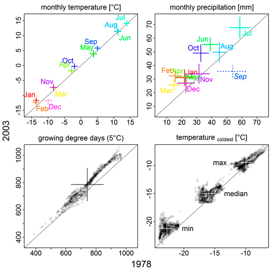
Fig. 1. Comparison of climate variables between 1978 and 2003. Monthly mean temperatures and precipitation sums, as well as growing degree days, were averaged over 10 years preceding the simulation year (1968–1977, 1993–2002); the mean temperature of the coldest month was averaged over 17 years preceding the simulation year (1961–1977 and 1986–2002, respectively). Plus signs indicate median (intersection) and standard deviation (length of the arms). Solid signs/plain text mean that values were significantly higher in 2003 than 1978, broken signs/italic text means the opposite (p < 0.001, Wilcoxon rank sum test); colour in the upper two panels is used to clarify label assignment. For growing degree days and coldest month mean temperatures, individual grid cell values are shown in addition to their median and standard deviation. See Supplementary file S1/Fig. S3 for more detailed information on monthly mean temperature and precipitation sums.

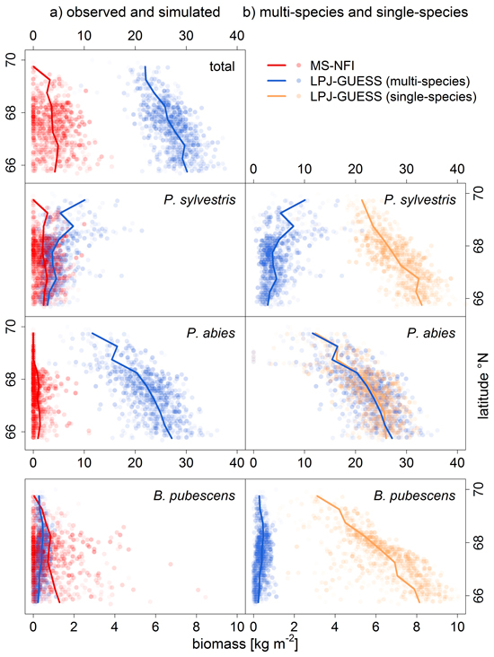
Fig. 2. Comparison of a) observed (MS-NFI data; red) and simulated biomass [kg m^–2] (LPJ-GUESS, multi-species run; blue), and, b) multi-species (i.e. with competition) and single-species (without competition; sandy) LPJ-GUESS runs, by latitude bands (lines are means within 0.5° latitude bands). Symbols are transparent to visualize the distribution of values. Note the different range of biomass values for Betula pubescens.

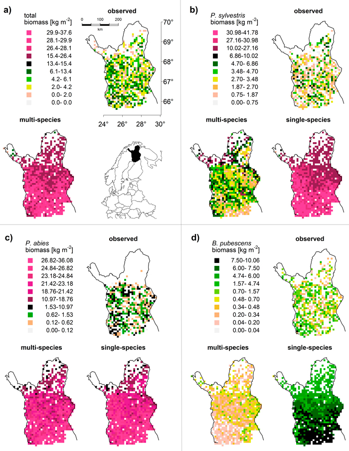
Fig. 3. Map comparison of (a) total and (b–d) species-specific biomass [kg m^–2]: observed data (MS-NFI, 2011) and results from multi-species and single-species LPJ-GUESS simulations (averaged over 1994–2003). To maximize visibility of spatial differences but retain comparability between observations and simulations, we used quantiles to define classes for each species and the total. This results in the irregular class spacing and reflects the different biomass distributions (cf. Fig. 2). “Natural” colours (white to black) cover the range of the observed values (i.e. the upper limit of the black class is always the maximum of the respective MS-NFI data); “artificial” colours (shades of magenta) cover the predictions that exceed the observed value range (model overestimation).

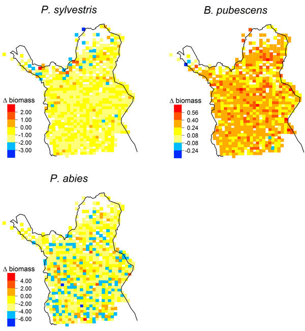
Fig. 4. Maps of simulated biomass changes [kg m^–2] from 1978 to 2003 (LPJ-GUESS, multi-species) for Pinus sylvestris, Picea abies and Betula pubescens.

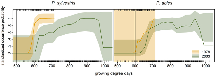
Fig. 5. Species-specific response curves of statistical occurrence models (cf. Schibalski et al. 2014, Fig. 7a) to growing degree days (averaged over the ten years preceding the inventory year, i.e. 1968–1977 and 1993–2002; given as rug plot in the upper panels: top 1978, bottom 2003). Vertical lines mark the bioclimatic limit used in LPJ-GUESS for the respective species (GDD_5,min, Suppl. file S1/Table S1). Transparent bootstrapped confidence bands (0.95) were calculated following the procedure detailed in Coutts (2011) and Coutts and Yokomizo (2014), using the boot.ci function in R (Canty and Ripley 2013). Note: The prevalence of Picea abies was very low in the 1978 dataset (7%) leading to the excessive bootstrapped confidence band (right).

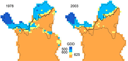
Fig. 6. Maps of growing degree days for 1978 (1968–1977) and 2003 (1993–2002) with treelines of Pinus sylvestris (solid) and Picea abies (broken). Treelines are defined as the marginal sites occupied by the respective species and had not changed between 1978 and 2003.