| Table 1. Average, maximum (Max), minimum (Min) and standard deviation (SD) of field variables in the field data in study area 2. | ||||
| Forest variable | Average | Max | Min | SD |
| Total volume, m3 ha–1 | 329.8 | 1160.8 | 33.2 | 220.5 |
| Volume of Scots pine, m3 ha–1 | 201.0 | 826.0 | 0.0 | 163.6 |
| Volume of Norway spruce, m3 ha–1 | 46.9 | 420.0 | 0.0 | 88.9 |
| Volume of Larix sp., m3 ha–1 | 39.9 | 1110.8 | 0.0 | 185.9 |
| Volume of broadleaved, m3 ha–1 | 42.0 | 352.6 | 0.0 | 84.7 |
| Mean diameter, cm | 22.9 | 55.4 | 13.9 | 7.7 |
| Mean height, m | 21.2 | 39.4 | 14.3 | 5.1 |
| Basal area, m2 ha–1 | 31.4 | 78.5 | 3.7 | 14.6 |
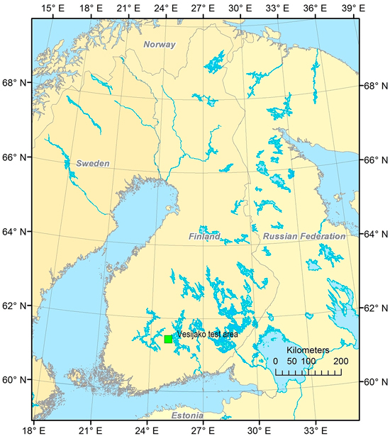
Fig. 1. Location of the study area.
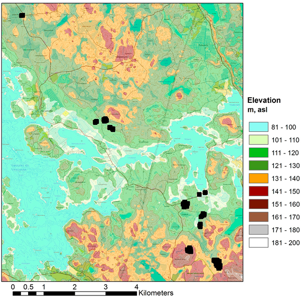
Fig. 2. Layout of the 11 test sites in the study area (topographic map and elevation model © National Land Survey of Finland, 2014).
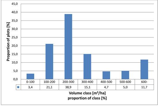
Fig. 3. Distribution of field plots in relation to growing stock volume.
| Table 2. Flight conditions and camera settings during the flights. Median irradiance was taken from Intersil ISL29004 irradiance measurements. Flight height is given from the ground level. | ||||||||
| Area | Date | Time (GPS) | Weather | Solar elevation | Sun azimuth | Median irrad | Exposure (ms) | Flight height (m) |
| v01 | 26.6 | 11:07 to 11:23 | cloudy | 50.91 | 199.22 | 2602 | 10 | 94 |
| v02 | 26.6 | 12:09 to 12:22 | cloudy | 47.38 | 219.63 | 4427 | 12 | 88 |
| v0304 | 25.6 | 10:38 to 10:51 | varying | 51.79 | 188.36 | variable | 6 | 85 |
| v05 | 25.6 | 09:26 to 09:40 | varying | 50.93 | 160.69 | variable | 6 | 86 |
| v0607 | 25.6 | 12:14 to 12:24 | cloudy | 47 | 221.30 | 3773 | 10 | 94 |
| v08 | 26.6 | 09:58 to 10:09 | sunny | 51.84 | 173.41 | 13894 | 10 | 86 |
| v09v10 | 25.6 | 13:51 to 14:12 | cloudy | 37.20 | 249.45 | 2546 | 8 | 84 |
| v11 | 26.6 | 08:49 to 08:58 | varying | 49.1 | 148.44 | 13982 | 10 | 83 |
| Table 3. Results of orientation processing; numbers of GCPs and images, reprojection errors and point density in points m–2. | ||||||
| Block | N GCP | RGB and FPI | RGB | |||
| N images | Reproj. error (pix) | N images | Reproj. error (pix) | Pointcloud points m–2 | ||
| v01 | 7 | 714 | 0.70 | 291 | 0.84 | 484 |
| v02 | 4 | 469 | 0.64 | 176 | 0.73 | 555 |
| v0304 | 9 | 758 | 0.60 | 281 | 0.70 | 711 |
| v05 | 5 | 717 | 0.68 | 292 | 0.89 | 601 |
| v06 | 3 | 193 | 0.91 | 76 | 1.10 | 510 |
| v07 | 4 | 176 | 1.63 | 68 | 2.56 | 524 |
| v08 | 5 | 421 | 0.73 | 178 | 0.99 | 538 |
| v09 | 4 | 280 | 0.57 | 109 | 0.66 | 621 |
| v10 | 3 | 182 | 0.65 | 70 | 0.88 | 484 |
| v11 | 4 | 469 | 0.478 | 469 | 0.478 | 833 |
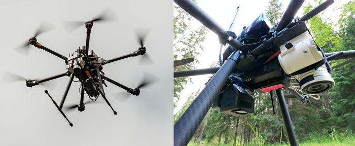
Fig. 4. UAV system (left) based on a Tarot 960 hexacopter and close-up of the sensor configuration (right) (Photographs by Tapio Huttunen).
| Table 4. Spectral settings of the FPI VIS/NIR. L0: central wavelength; FWHM: full width at half maximum. |
| L0 (nm): 507.60, 509.50, 514.50, 520.80, 529.00, 537.40, 545.80, 554.40, 562.70, 574.20, 583.60, 590.40, 598.80, 605.70, 617.50, 630.70, 644.20, 657.20, 670.10, 677.80, 691.10, 698.40, 705.30, 711.10, 717.90, 731.30, 738.50, 751.50, 763.70, 778.50, 794.00, 806.30, 819.70, 833.70, 845.80, 859.10, 872.80, 885.60 |
| FWHM (nm): 11.2, 13.6, 19.4, 21.8, 22.6, 20.7, 22.0, 22.2, 22.1, 21.6, 18.0, 19.8, 22.7, 27.8, 29.3, 29.9, 26.9, 30.3, 28.5, 27.8, 30.7, 28.3, 25.4, 26.6, 27.5, 28.2, 27.4, 27.5, 30.5, 29.5, 25.9, 27.3, 29.9, 28.0, 28.9, 32.0, 30.8, 27.9 |
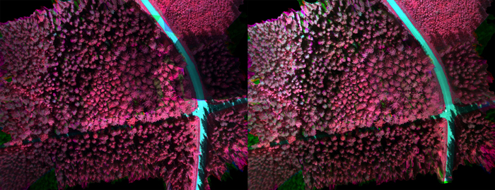
Fig. 5a. Original image mosaic (left) acquired in weather conditions changing from cloudy to clear during imaging flight and radiometrically calibrated mosaic (right).
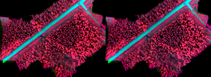
Fig. 5b. Original image mosaic (left) acquired in uniform cloudy weather conditions during imaging flight and radiometrically calibrated mosaic (right).
| Table 5a. Estimation results, non-calibrated HS-mosaic, common features. | ||||||||
| Variable | k | g | RMSE (%) | Bias (%) | n.3D.feat. | n.HS.feat. | n.RGB.feat. | n.feat. |
| D | 3 | 2.6 | 18.32 | –2.17 | 7 | 9 | 1 | 17 |
| H | 3 | 2.6 | 8.67 | –0.40 | 7 | 9 | 1 | 17 |
| Volume | 3 | 2.6 | 31.47 | –0.59 | 7 | 9 | 1 | 17 |
| vol.pine | 3 | 2.6 | 45.66 | 0.54 | 7 | 9 | 1 | 17 |
| vol.spruce | 3 | 2.6 | 97.58 | 1.18 | 7 | 9 | 1 | 17 |
| vol.larch | 3 | 2.6 | 91.53 | –1.31 | 7 | 9 | 1 | 17 |
| vol.broadleaved | 3 | 2.6 | 63.98 | –7.26 | 7 | 9 | 1 | 17 |
| n.3D.feat. = number of 3D features; n.HS.feat. = number of hyperspectral features; n.RGB.feat. = number of RGB features; n.feat. = total number of selected features. | ||||||||
| Table 5b. Estimation results, non-calibrated HS-mosaic, individual features. | ||||||||
| Variable | k | g | RMSE (%) | Bias (%) | n.3D.feat. | n.HS.feat. | n.RGB.feat. | n.feat. |
| D | 5 | 0.7 | 14.71 | –0.52 | 4 | 11 | 0 | 15 |
| H | 5 | 1.3 | 7.36 | –0.07 | 4 | 5 | 1 | 10 |
| Volume | 5 | 2.9 | 22.65 | 0.00 | 8 | 7 | 1 | 16 |
| vol.pine | 3 | 0.7 | 40.02 | –0.03 | 4 | 5 | 1 | 10 |
| vol.spruce | 6 | 2.0 | 65.06 | 0.02 | 6 | 18 | 1 | 25 |
| vol.larch | 3 | 3.0 | 45.67 | –3.00 | 6 | 11 | 3 | 20 |
| vol.broadleaved | 5 | 2.0 | 44.52 | 0.04 | 5 | 14 | 2 | 21 |
| n.3D.feat. = number of 3D features; n.HS.feat. = number of hyperspectral features; n.RGB.feat. = number of RGB features; n.feat. = total number of selected features. | ||||||||
| Table 5c. Estimation results, calibrated HS-mosaic, common features. | ||||||||
| Variable | k | g | RMSE (%) | Bias (%) | n.3D.feat. | n.HS.feat. | n.RGB.feat. | n.feat. |
| D | 5 | 2.9 | 19.19 | –1.76 | 9 | 6 | 1 | 16 |
| H | 5 | 2.9 | 9.05 | –0.43 | 9 | 6 | 1 | 16 |
| Volume | 5 | 2.9 | 26.93 | –1.60 | 9 | 6 | 1 | 16 |
| vol.pine | 5 | 2.9 | 41.94 | 0.66 | 9 | 6 | 1 | 16 |
| vol.spruce | 5 | 2.9 | 77.52 | –9.68 | 9 | 6 | 1 | 16 |
| vol.larch | 5 | 2.9 | 60.22 | 2.30 | 9 | 6 | 1 | 16 |
| vol.broadleaved | 5 | 2.9 | 81.98 | –7.10 | 9 | 6 | 1 | 16 |
| n.3D.feat. = number of 3D features; n.HS.feat. = number of hyperspectral features; n.RGB.feat. = number of RGB features; n.feat. = total number of selected features. | ||||||||
| Table 5d. Estimation results, calibrated HS-mosaic, individual features. | ||||||||
| Variable | k | g | RMSE (%) | Bias (%) | n.3D.feat. | n.HS.feat. | n.RGB.feat. | n.feat. |
| D | 5 | 2.0 | 15.20 | –1.76 | 4 | 8 | 0 | 12 |
| H | 6 | 1.5 | 7.50 | –0.14 | 6 | 5 | 3 | 14 |
| Volume | 5 | 2.5 | 23.96 | 0.00 | 8 | 4 | 2 | 14 |
| vol.pine | 5 | 2.0 | 34.51 | 0.00 | 11 | 8 | 0 | 19 |
| vol.spruce | 5 | 2.3 | 57.16 | –0.01 | 6 | 7 | 2 | 15 |
| vol.larch | 3 | 2.6 | 51.07 | –0.29 | 5 | 5 | 2 | 12 |
| vol.broadleaved | 4 | 2.1 | 42.00 | –1.38 | 7 | 13 | 2 | 22 |
| n.3D.feat. = number of 3D features; n.HS.feat. = number of hyperspectral features; n.RGB.feat. = number of RGB features; n.feat. = total number of selected features. | ||||||||
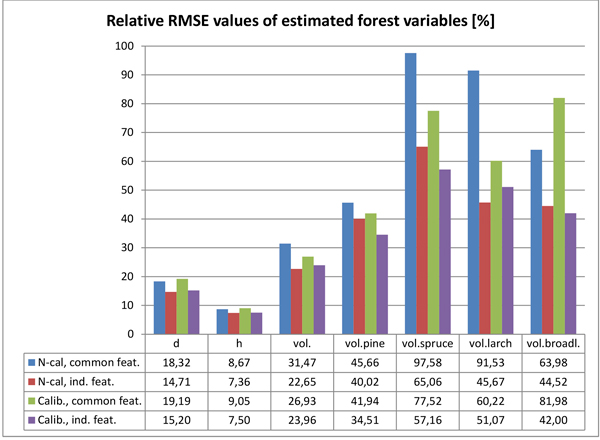
Fig. 6. Relative RMSEs of the estimated forest variables with the tested two calibration options (N-cal = non calibrated; Calib. = calibrated imagery) and feature selection strategies (common features for all variables vs. individual feature set for each variable).
| Table 6. Estimation results, calibrated HS-mosaic, features optimized for tree species volumes. | ||||||||
| Variable | k | g | RMSE (%) | Bias (%) | n.3D.feat. | n.HS.feat. | n.RGB.feat. | n.feat. |
| vol.pine | 5 | 3 | 40.63 | –0.43 | 9 | 12 | 3 | 24 |
| vol.spruce | 5 | 3 | 75.78 | –1.56 | 9 | 12 | 3 | 24 |
| vol.broadleaved | 5 | 3 | 50.05 | –0.48 | 9 | 12 | 3 | 24 |
| n.3D.feat. = number of 3D features; n.HS.feat. = number of hyperspectral features; n.RGB.feat. = number of RGB features; n.feat. = total number of selected features. | ||||||||