| Table 1. The general description of simulated annealing (SA) algorithm. |
| 1: Set SA parameters: start temperature (st), the final temperature (ft), the cooling rate (cr) and the number of iterations allowed at each temperature (nrep), and select the search strategy to generate candidate solution. 2: Generate an initial feasible solution by assigning a random prescription to each management unit (MU). Set this solution as the current (S) and best solution (S*). 3: Compute the objective function value of S. 4: Generate a candidate solution (S’) based on the current solution S by randomly selecting n MUs according to the search strategies, and then randomly change (i.e., Method 1 and Method 3) or just exchange their prescriptions (i.e., Method 2) of different MUs. 5: Check the conformity of the new candidate solution (S’) to constraints 4 and 5 in the planning formulation (see Section 2.1 for details). If feasible, go to step 6; otherwise, return to step 4. 6: Evaluate the feasibility of candidate solution S’ against the harvest even-flow (i.e., Eqs. 9–10), ending inventory (i.e., Eq. 11) and adjacency constraints (i.e., Eqs. 12–13; see Section 2.1 for details). If infeasible, reject the candidate solution, and go back to step 4. 7: Compute the objective function value of S’. 8: If the objective function value of S’ is larger than that of S*, go to step 9. Otherwise, go to step 10. 9: Let S = S’ and S* = S’, and move to step 10. 10: Evaluate the acceptability of the candidate solution S’ with respect to the objective function value, i.e., compare the result between the value of Boltzman formula (i.e., e(–∆E/t)) and a random number that varies between 0 and 1, in which ∆E is the difference between S’ and S*, and t is the current temperature. 11: If the non-improving solution is rejected, then directly go to step 12. Otherwise, let S = S’, and go to step 12. 12: If nrep is not reached, increase nrep by one, and go back to step 4. Otherwise, cool the temperature according to cooling rate cr and reset nrep to zero, and go to step 13. 13: If ft is not reached, then go back to step 4. Otherwise, output the best solution S*. |
| Table 2. The statistical results of 1000 independent objective function values (106 m3) of the three planning problems for each hypothetical forest dataset when using three different neighborhood search techniques of simulated annealing (SA). The largest minimum objective function value for each planning scenario is highlighted in italic, the maximum objective function value is highlighted in boldface, the maximum mean objective function value is highlighted with a shadow, and the smallest standard deviation (SD) value is highlighted with underline. Method 1 represents the standard version of SA using 1-opt moves, Method 2 represents the exchange version of SA using 2-opt moves, and Method 3 represents the change version of SA using 2-opt moves. NON represents the non-spatial planning problems, URM represents the unit restriction model, ARM represents the area restriction model. | ||||||||||||||
| Forest | Model | Method 1 | Method 2 | Method 3 | ||||||||||
| Min. | Max. | Mean | SD | Min. | Max. | Mean | SD | Min. | Max. | Mean | SD | |||
| 400 | NON | 0.558 | 0.623 | 0.572 | 0.013 | 0.561 | 0.634 | 0.574 | 0.013 | 0.560 | 0.638 | 0.575 | 0.014 | |
| ARM | 0.553 | 0.622 | 0.567 | 0.013 | 0.555 | 0.630 | 0.568 | 0.012 | 0.556 | 0.637 | 0.568 | 0.013 | ||
| URM | 0.457 | 0.598 | 0.486 | 0.023 | 0.460 | 0.598 | 0.488 | 0.023 | 0.463 | 0.612 | 0.489 | 0.024 | ||
| 1600 | NON | 2.217 | 2.602 | 2.267 | 0.083 | 2.222 | 2.616 | 2.266 | 0.074 | 2.224 | 2.635 | 2.267 | 0.072 | |
| ARM | 2.127 | 2.577 | 2.201 | 0.080 | 2.136 | 2.587 | 2.197 | 0.064 | 2.137 | 2.607 | 2.202 | 0.066 | ||
| URM | 1.714 | 2.420 | 1.847 | 0.084 | 1.706 | 2.441 | 1.848 | 0.081 | 1.720 | 2.448 | 1.855 | 0.083 | ||
| 3600 | NON | 4.887 | 5.744 | 5.041 | 0.260 | 4.894 | 5.752 | 5.005 | 0.208 | 4.892 | 5.800 | 4.980 | 0.168 | |
| ARM | 4.741 | 5.683 | 4.910 | 0.218 | 4.757 | 5.673 | 4.872 | 0.139 | 4.766 | 5.727 | 4.897 | 0.180 | ||
| URM | 3.859 | 4.692 | 4.288 | 0.174 | 3.814 | 4.687 | 4.280 | 0.182 | 3.866 | 5.338 | 4.285 | 0.181 | ||
| 6400 | NON | 8.790 | 10.237 | 9.102 | 0.508 | 8.794 | 10.482 | 9.042 | 0.488 | 8.809 | 10.499 | 9.025 | 0.457 | |
| ARM | 8.258 | 10.086 | 8.778 | 0.579 | 8.306 | 10.303 | 8.603 | 0.440 | 8.331 | 10.304 | 8.617 | 0.437 | ||
| URM | 6.860 | 8.183 | 7.631 | 0.298 | 6.862 | 8.172 | 7.660 | 0.299 | 6.897 | 8.154 | 7.647 | 0.283 | ||
| 10000 | NON | 13.675 | 15.620 | 14.319 | 0.795 | 13.695 | 16.212 | 14.141 | 0.832 | 13.719 | 16.274 | 14.178 | 0.863 | |
| ARM | 12.782 | 15.475 | 13.946 | 1.010 | 12.913 | 15.983 | 13.490 | 0.856 | 12.893 | 15.885 | 13.555 | 0.870 | ||
| URM | 10.705 | 12.711 | 12.007 | 0.439 | 10.873 | 12.724 | 12.028 | 0.433 | 10.887 | 12.690 | 12.050 | 0.418 | ||
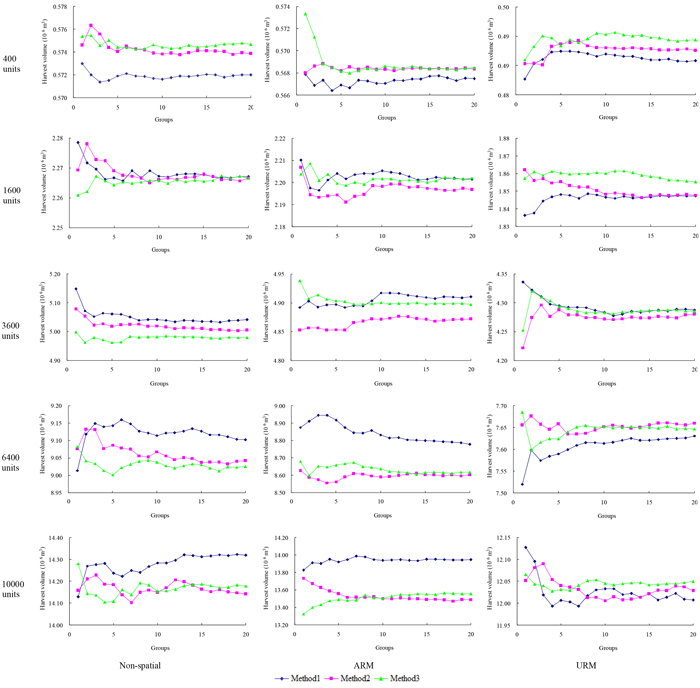
Fig. 1. The development of mean objective function value within each group of the three planning problems for the five hypothetical forest datasets when employed using three different neighborhood search techniques of simulated annealing (SA). Method 1 represents the standard version of SA using 1-opt moves, Method 2 represents the exchange version of SA using 2-opt moves, and Method 3 represents the change version of SA using 2-opt moves. Non-spatial represents the non-spatial planning problems, URM represents the unit restriction model, ARM represents the area restriction model. View larger in new window/tab.
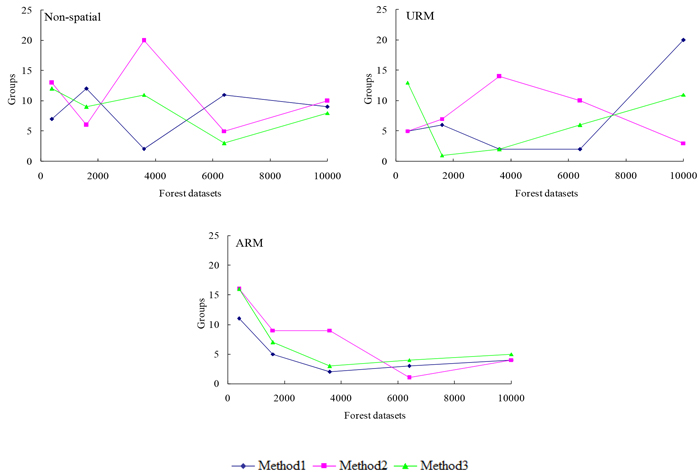
Fig. 2. The development of the group orders in which the maximum objective function values were obtained for the alternative planning problems related to the number of management units within a forest dataset, when using three different neighborhood search techniques of simulated annealing (SA). Method 1 represents the standard version of SA using 1-opt moves, Method 2 represents the exchange version of SA using 2-opt moves, and Method 3 represents the change version of SA using 2-opt moves. Non-spatial represents the non-spatial planning problems, URM represents the unit restriction model, ARM represents the area restriction model. View larger in new window/tab.
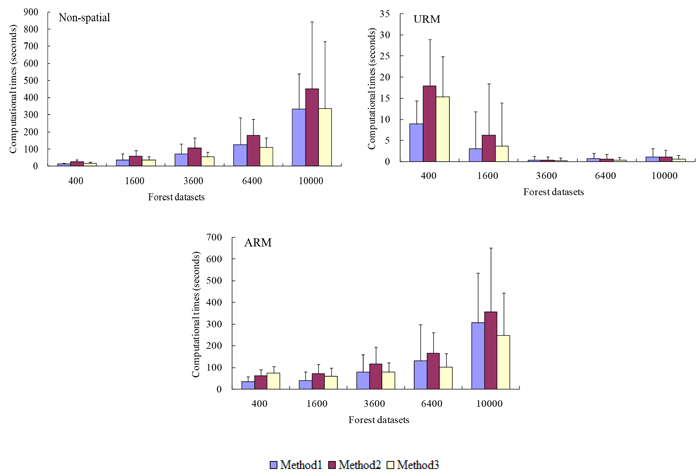
Fig. 3. The mean and standard deviation of computation time for alternative planning problems related to the number of management units within a forest dataset, when using three different neighborhood search techniques of simulated annealing (SA). Method 1 represents the standard version of SA using 1-opt moves, Method 2 represents the exchange version of SA using 2-opt moves, and Method 3 represents the change version of SA using 2-opt moves. Non-spatial represents the non-spatial planning problems, URM represents the unit restriction model, ARM represents the area restriction model. View larger in new window/tab.