| Table 1. The generalized algebraic difference approach models fitted to dominant height time series of beech according to Sharma et al. (2011). | |
| Base model | Generalized algebraic difference approach model |
 | |
| Table 2. Parameter estimates and their t-values of the fitted models. Models fit statistics: mean absolute residual (MR), residual standard error (RSE), root mean squared error (RMSE), Akaike information criterion (AIC), adjusted R2-value (McNemar’s method), and variance components of the random effects (VAR). | |||||||
| Chapman-Richards | Hossfeld | Hossfeld I | King-Prodan | Log-logistic | Sloboda | Strand | |
| Parameter estimates | |||||||
| b1 | 0.0227 | 43.7466 | 0.0228 | 1.576 | 43.803 | 52.9402 | 0.1789 |
| b2 | –9.8636 | 121.078 | –0.0054 | 118.678 | –104.29 | 0.2502 | –0.0034 |
| b3 | 42.6561 | 1.5954 | –5281.7 | –1.6153 | 0.6489 | 2.2777 | |
| Estimate t-values | |||||||
| b1 | 16.88 | 10.36 | 11.47 | 37.15 | 11.83 | 7.8 | 8.48 |
| b2 | 1.91 | 2.65 | 4.7 | 2.17 | 0.06 | 7.57 | 2.03 |
| b3 | 2.23 | 37.81 | 2.03 | 38.12 | 12.98 | 15.7 | |
| Model statistics | |||||||
| MR (m) | 0.48 | 0.51 | 0.72 | 0.52 | 0.53 | 0.49 | 0.51 |
| RSE (m) | 0.6 | 0.65 | 0.83 | 0.65 | 0.67 | 0.63 | 0.64 |
| RMSE (m) | 0.6 | 0.64 | 0.82 | 0.65 | 0.66 | 0.62 | 0.64 |
| AIC | 660.3 | 685.3 | 835 | 686.9 | 694.3 | 656.8 | 677.7 |
| Adj. R2 | 0.9963 | 0.9956 | 0.9958 | 0.9956 | 0.9954 | 0.9959 | 0.9958 |
| VAR (tree) | 0.317 | 1.125 | 0.133 | 0.013 | 0.432 | 0.721 | 0.009 |
| VAR (stand) | 0.011 | 1.965 | 2.231 | 2.023 | 0.414 | 0.168 | 0.377 |
| VAR (residual) | 0.367 | 0.418 | 0.553 | 0.422 | 0.441 | 0.384 | 0.409 |
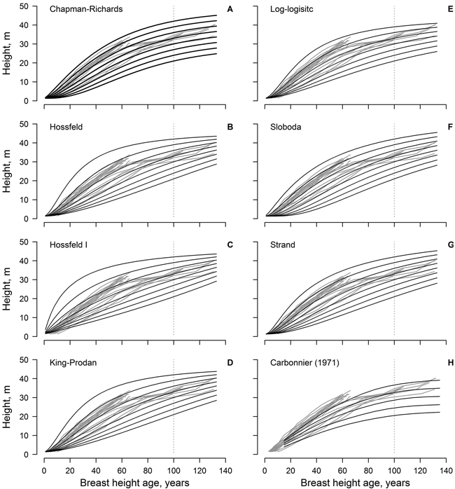
Fig. 1. The non-linear dominant height models (black lines) fitted to the observed data (grey lines, each line represent single tree); model predictions are for 3 m site index intervals for the range 21–42 m (A–G). Panel H show the height growth of beech in southern Sweden according to Carbonnier (1971); black line show site indices in 4 m intervals for the range 20–36 m.
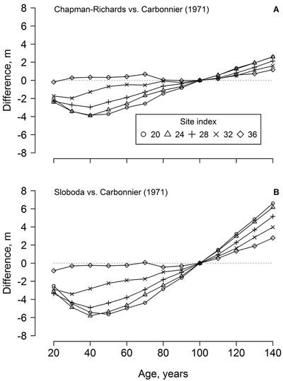
Fig. 2. The differences between beech dominant height predicted by the developed Chapman-Richards (A) and Sloboda (B) models in the western part of Latvia and yield tables for southern Sweden (cf. Carbonnier 1971) according to stand age and site index.