| Table 1. Site and stand characteristics of the experiments and total amount of the applied fertilisers. | ||||||||||||
| Exp. | Lat. °N | Long. °E | Tempsum d.d. (>5 °C) | Tree species | Started at | Stand age at 2009 | SI a), m | Prod a) , m3 ha–1 a–1 | N, kg ha–1 | P, kg ha–1 | Lime, kg ha–1 | Soil texture b) |
| 25 | 61.817 | 29.329 | 1239 | Pine | 1958 | 84 | 27.9 | 7.4 | 1676 | 149 | 6000 | SL |
| 33 | 61.875 | 29.343 | 1234 | Pine | 1958 | 70 | 29.3 | 5.9 | 1908 | 120 | 6000 | LS |
| 35 | 62.409 | 28.707 | 1168 | Spruce | 1958 | 77 | 18.3 | 8.3 | 714 | 144 | 6000 | SL |
| 36 | 62.409 | 28.710 | 1168 | Spruce | 1958 | 77 | 19.9 | 8.5 | 714 | 144 | 6000 | SL |
| 37 | 61.415 | 28.545 | 1240 | Pine | 1958 | 75 | 20.0 | 7.4 | 714 | 109 | 6000 | LS |
| 38 | 61.416 | 28.542 | 1233 | Pine | 1958 | 75 | 21.5 | 8.2 | 714 | 109 | 6000 | S |
| 52 | 62.024 | 24.811 | 1154 | Pine | 1959 | 58 | 25.9 | 8.1 | 1496 | 149 | 6000 | LS |
| 55 | 61.662 | 29.304 | 1170 | Pine | 1959 | 65 | 26.1 | 9.8 | 534 | 69 | 6000 | SL |
| 56 | 62.927 | 25.607 | 1025 | Pine | 1959 | 76 | 22.8 | 4.5 | 1496 | 149 | 6000 | SL |
| 57 | 62.935 | 25.678 | 1020 | Spruce | 1959 | 77 | 19.4 | 5.9 | 1496 | 149 | 6000 | SL |
| 58 | 62.935 | 25.677 | 1024 | Spruce | 1959 | 77 | 21.5 | 6.9 | 1496 | 149 | 6000 | SL |
| 60 | 62.930 | 25.666 | 1020 | Spruce | 1959 | 77 | 23.0 | 7.7 | 1136 | 109 | 6000 | SL |
| 64 | 61.493 | 29.066 | 1215 | Pine | 1959 | 90 | 22.0 | 5.3 | 714 | 109 | 6000 | LS |
| 67 | 61.537 | 29.062 | 1160 | Pine | 1959 | 70 | 21.1 | 9.3 | 714 | 109 | 6000 | SL |
| 68 | 61.956 | 27.575 | 1147 | Pine | 1959 | 84 | 21.5 | 7.6 | 1404 | 149 | 6000 | S |
| 73 | 62.759 | 24.747 | 1034 | Pine | 1959 | 55 | 25.9 | 8.0 | 1254 | 160 | 6000 | SL |
| 75 | 62.913 | 24.571 | 1028 | Pine | 1959 | 54 | 25.3 | 4.9 | 742 | 109 | 6000 | SL |
| 76 | 62.912 | 24.570 | 1028 | Pine | 1959 | 54 | 26.3 | 5.2 | 742 | 109 | 6000 | SL |
| 77 | 62.911 | 24.568 | 1028 | Pine | 1959 | 54 | 23.3 | 4.1 | 742 | 109 | 6000 | SL |
| 82 | 63.300 | 25.340 | 999 | Pine | 1959 | 54 | 17.6 | 3.7 | 965 | 193 | 6000 | SL |
| 97 | 62.574 | 24.119 | 1074 | Pine | 1960 | 61 | 24.8 | 8.5 | 742 | 193 | 6000 | LS |
| 98 | 62.579 | 24.125 | 1074 | Pine | 1959 | 60 | 24.5 | 6.9 | 1356 | 69 | 6000 | SL |
| 103 | 63.215 | 24.624 | 1006 | Pine | 1960 | 58 | 22.2 | 4.2 | 742 | 109 | 6000 | LS |
| 106 | 63.389 | 24.300 | 1013 | Pine | 1960 | 73 | 15.0 | 3.0 | 1136 | 120 | 6000 | LS |
| 107 | 63.095 | 24.294 | 1013 | Pine | 1960 | 63 | 18.0 | 2.6 | 742 | 153 | 6000 | LS |
| 113 | 61.172 | 26.050 | 1251 | Spruce | 1961 | 58 | 28.4 | 12.8 | 1486 | 193 | 6000 | SL |
| 135 | 67.250 | 23.869 | 791 | Pine | 1961 | 87 | 17.6 | 4.6 | 1194 | 120 | 6000 | SL |
| 155 | 61.169 | 26.048 | 1250 | Spruce | 1962 | 59 | 28.2 | 13.4 | 1074 | 160 | 6000 | SL |
| 157 | 61.111 | 26.026 | 1229 | Pine | 1962 | 62 | 24.2 | 7.1 | 1317 | 160 | 5000 | LS |
| 194 | 66.855 | 27.133 | 754 | Spruce | 1964 | 74 | 19.5 | 1.5 | 1110 | 160 | 6000 | SL |
| a) SI is H100 and Prod is the mean annual stem volume production for plots not fertilised with N (4 per experiment). b) Soil texture classes: S = sand, LS = loamy sand and SL = sandy loam. | ||||||||||||
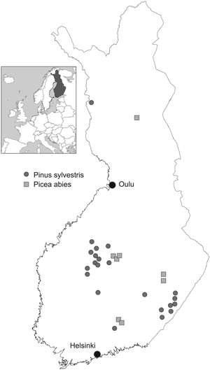
Fig. 1. Fertilisation experiments.
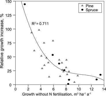
Fig. 2. Relative increase in stand production caused by nitrogen fertilisation as a function of mean annual production on unfertilised (no N) plots.
| Table 2. Concentrations of elements by fertilisation treatment. Covariates in the ANOVA were effective temperature sum, tree species, i.e. pine (0//1), and mean thickness of the organic layer on plots not fertilised with N. | |||||||||
| Variable b) | Treatments a) | ||||||||
| Cntrl | N | P | L | NP | NL | PL | NPL | F value c) | |
| Organic layer | |||||||||
| Ctot, g kg–1 | 442a | 443a | 428ab | 362e | 444a | 403bc | 370de | 396cd | 28.4 |
| Ntot, g kg–1 | 12.6b | 15.2a | 12.1b | 10.5c | 15.1a | 14.4a | 10.9c | 14.3a | 60.0 |
| C/N | 35.7a | 29.6b | 38.1a | 35.2a | 29.8b | 28.7b | 34.9a | 28.4b | 66.7 |
| Catot, mg kg–1 | 2823c | 2960c | 4261c | 8246b | 4378c | 9420ab | 10471a | 10525a | 87.2 |
| K tot, mg kg–1 | 769a | 622cd | 734ab | 693bc | 597d | 620d | 738ab | 641cd | 13.6 |
| Mgtot, mg kg–1 | 396b | 502b | 386b | 1841a | 491b | 2019a | 2104a | 2231a | 30.5 |
| Ptot, mg kg–1 | 796b | 757bc | 946a | 706c | 912a | 714bc | 951a | 966a | 33.4 |
| pHCaCl2 | 3.22d | 3.21d | 3.38bc | 4.06a | 3.35cd | 4.07a | 4.19a | 4.18a | 191 |
| CaAAA, mg kg–1 | 1964d | 2014d | 2902cd | 5157b | 2963c | 5922ab | 6212a | 6255a | 118 |
| KAAA, mg kg–1 | 784a | 581c | 752ab | 687b | 583c | 583c | 704b | 570c | 28.1 |
| MgAAA, mg kg–1 | 273b | 347b | 252b | 773a | 337b | 904a | 782a | 912a | 45.3 |
| PAAA, mg kg–1 | 230bc | 179de | 270a | 184de | 232bc | 157e | 246ab | 212bcd | 25.9 |
| Mineral soil | |||||||||
| C, g kg–1 | 25.9bc | 30.5ab | 25.3c | 29.2abc | 29.6abc | 28.4abc | 27.5abc | 31.8a | 4.39 |
| Ntot g kg–1 | 1.03cd | 1.25ab | 1.02d | 1.13bcd | 1.20abcd | 1.21abc | 1.05cd | 1.34a | 7.80 |
| C/N | 25.9ab | 24.6bc | 25.1abc | 26.1ab | 24.8bc | 23.7c | 27.0a | 24.4bc | 5.51 |
| pHCaCl2 | 3.99b | 3.80b | 3.92b | 4.68a | 3.81b | 4.37a | 4.71a | 4.55a | 74.1 |
| CaAAA, mg kg–1 | 63c | 78c | 120c | 680a | 105c | 474b | 694a | 683a | 52.2 |
| KAAA, mg kg–1 | 31.3a | 30.2a | 32.7a | 33.2a | 29.6a | 27.8a | 32.4a | 30.1a | 2.17 |
| MgAAA, mg kg–1 | 11.1b | 15.3b | 12.9b | 83.5a | 16.3b | 80.7a | 81.1a | 86.0a | 42.5 |
| PAAA, mg kg–1 | 9.6c | 8.8cd | 12.4a | 7.1de | 11.8ab | 6.1e | 10.0bc | 9.2cd | 20.3 |
| a) Cntrl = control, N = nitrogen fertilisation, P = phosphorus fertilisation, L = liming. b) AAA = acid ammonium acetate extraction, tot = dry combustion concentration. c) F value from mixed model ANOVA with covariates. If F7,200 > 3.64, then p < 0.001. | |||||||||
| Table 3. Amounts of elements by fertilisation treatment. Potential covariates in the ANOVA were effective temperature sum, tree species, i.e. pine (0/1), and mean thickness of the organic layer on plots not fertilised with N. | |||||||||
| Variable b) | Treatments a) | ||||||||
| Cntrl | N | P | L | NP | NL | PL | NPL | F value c) | |
| Organic layer | |||||||||
| Ctot, Mg ha–1 | 16.8b | 22.8a | 17.5b | 16.0b | 22.5a | 21.0a | 16.4b | 20.5a | 25.2 |
| Ntot, kg ha–1 | 488b | 778a | 496b | 468b | 764a | 741a | 485b | 734a | 58.9 |
| Catot, kg ha–1 | 112d | 150cd | 177cd | 373b | 221c | 488a | 485a | 545a | 64.9 |
| Ptot, kg ha–1 | 30.5e | 38.2cd | 38.8cd | 31.7e | 46.1ab | 36.8d | 42.2bc | 49.8a | 35.6 |
| Mineral soil | |||||||||
| Ctot, Mg ha–1 | 20.8bc | 24.3ab | 20.3c | 22.6abc | 23.7ab | 22.7abc | 22.6abc | 24.5a | 5.28 |
| Ntot, kg ha–1 | 842d | 998a | 822d | 883bcd | 961abc | 977ab | 860c | 1023a | 9.38 |
| Org. + min. soil | |||||||||
| CaAAA, kg ha–1 | 127d | 162d | 214d | 771bc | 233d | 693c | 862ab | 870a | 88.8 |
| PAAA, kg ha–1 | 16.4cd | 16.1cd | 21.2a | 14.0de | 21.5a | 13.2e | 19.4ab | 18.5bc | 33.3 |
| a) Cntrl = control, N = nitrogen fertilisation, P = phosphorus fertilisation, L = liming. b) AAA = acid ammonium acetate extraction, tot = dry combustion concentration. c) F value from mixed model ANOVA with covariates. If F7,200 > 3.64, then p < 0.001. | |||||||||
| Table 4. Regression equations for total concentrations of elements as a function of cumulative amounts of fertilisers, and site and tree-stand properties. All coefficients are statistically significant (p < 0.05). | ||||||||
| Dependent variables | ||||||||
| Organic layer | Mineral soil 0–10 cm | |||||||
| Independent variables a) | Ntot g kg–1 | C/N | lnCatot mg kg–1 | Ktot mg kg–1 | Ptot mg kg–1 | ln(Ntot+1) g kg–1 | C/N | |
| Constant b) | –4.61 | 50.9 | 7.16 | 237 | 316 | –.278 | 22.3 | |
| N, Mg ha–1 | 3.07 | –5.76 | –116 | .0820 | –1.40 | |||
| P, kg ha–1 | .000849 | 1.47 | ||||||
| Lime, Mg ha–1 | –.208 | .167 | ||||||
| Ol. thickn., cm | 1.22 | |||||||
| Stand age, a | .0978 | .00701 | 5.77 | 5.56 | ||||
| Pine (0/1) | –2.24 | 8.09 | –129 | –.278 | 3.10 | |||
| Tempsum, d.d. | .00703 | –.0197 | .000896 | |||||
| Fines, % | .0107 | 3.47 | 4.72 | .00680 | ||||
| Stones, % | .0531 | |||||||
| R2 (obs./pred.) | .667 | .738 | .688 | .441 | .619 | .667 | .256 | |
| a) N = cumulative amount of fertilised nitrogen, P = cumulative amount of fertilised phosphorus, Lime = cumulative amount of spread lime, Ol. thickn. = mean organic layer thickness on plots not fertilised with nitrogen, Stand age = stand age at year 2009, Pine = 1, if pine, 0 if spruce, Tempsum = average effective temperature sum, Fines = sum of clay + silt, i.e. under 63 µm fraction, Stones = Volumetric percentage of stones. b) In the logaritmic models the constant has been adjusted to yield the original arithmetic mean by adding a residual variance of the regression model, constant + sf2/2. | ||||||||
| Table 5. Regression equations for pH and concentrations of elements extracted with acid ammonium acetate as a function of cumulative amounts of fertilisers and site and tree-stand properties. All coefficients are statistically significant. | |||||||||||
| Dependent variables | |||||||||||
| Organic layer | Mineral soil 0–10 cm | ||||||||||
| Independent variables a) | pHCaCl2 | CaAAA mg kg–1 | KAAA mg kg–1 | PAAA mg kg–1 | pHCaCl2 | lnCaAAA mg kg–1 | lnKAAA mg kg–1 | lnPAAA mg kg–1 | |||
| Constant b) | 3.88 | 2879 | 932 | 163 | 3.31 | 4.00 | 2.29 | 1.97 | |||
| N, Mg ha–1 | –.0874 | –135 | –33.7 | –.248 | –.207 | ||||||
| P, kg ha–1 | .412 | .00295 | |||||||||
| Lime, Mg ha–1 | .139 | .562 | –6.46 | –4.75 | .114 | .360 | –.0464 | ||||
| Ol. thickn., cm | –.120 | –.240 | –.163 | –.150 | |||||||
| Stand age, a | 5.27 | ||||||||||
| Pine (0/1) | –.342 | –1222 | .421 | ||||||||
| Tempsum, d.d. | –.495 | .000855 | |||||||||
| Fines, % | 1.96 | .0101 | .0292 | .0189 | .0231 | ||||||
| Stones, % | .00565 | ||||||||||
| R2 (obs./pred.) | .811 | .756 | .442 | .346 | .646 | .575 | .583 | .540 | |||
| a) N = cumulative amount of fertilised nitrogen, P = cumulative amount of fertilised phosphorus, Lime = cumulative amount of spread lime, Ol. thickn. = mean organic layer thickness on plots not fertilised with nitrogen, Stand age = stand age at year 2009, Pine = 1, if pine, 0 if spruce, Tempsum = average effective temperature sum, Fines = sum of clay + silt, i.e. under 63 µm fraction, Stones = Volumetric percentage of stones. b) In the logaritmic models the constant has been adjusted to yield the original arithmetic mean by adding a residual variance of the regression model, constant + sf2/2. | |||||||||||
| Table 6. Regression equations for total amounts of elements as a function of cumulative amounts of fertilisers, and site and tree-stand properties. All coefficients are statistically significant. | |||||||
| Dependent variables | |||||||
| Organic layer | Mineral soil 0–10 cm | ||||||
| Independent variables a) | Ctot kg ha–1 | Ntot kg ha–1 | lnCatot kg ha–1 | Ktot kg ha–1 | Ptot kg ha–1 | lnCtot, kg ha–1 | lnNtot, kg ha–1 |
| Constant b) | 8898 | 579 | 5.01 | 35.7 | 39.7 | 8.21 | 5.28 |
| N, Mg ha–1 | 4476 | 245 | .139 | 6.31 | .104 | .158 | |
| P, kg ha–1 | .000829 | .0727 | |||||
| Lime, Mg ha–1 | –229 | –4.10 | .181 | .325 | .00769 | ||
| Tempsum, d.d. | .00148 | .00134 | |||||
| Ol. thickn., cm | 2562 | ||||||
| Fines, % | .00957 | .00845 | |||||
| Pine (0/1) | –125 | –.338 | –8.01 | –.278 | –.405 | ||
| R2 (obs./pred.) | .400 | .544 | .593 | .192 | .468 | .578 | .641 |
| a) N = cumulative amount of fertilised nitrogen, P = cumulative amount of fertilised phosphorus, Lime = cumulative amount of spread lime, Ol. thickn. = mean organic layer thickness on plots not fertilised with nitrogen, Pine = 1, if pine, 0 if spruce, Tempsum = average effective temperature sum, Fines = sum of clay + silt, i.e. under 63 µm fraction. b) In the logaritmic models the constant has been adjusted to yield the original arithmetic mean by adding a residual variance of the regression model, constant + sf2/2. | |||||||
| Table 7. Regression equations for elemental amounts extracted with acid ammoníum acetate as a function of cumulative amounts of fertilisers and site and tree-stand properties. All coefficients are statistically significant. | ||||||||||
| Dependent variables | ||||||||||
| Organic layer | Mineral soil 0–10 cm | |||||||||
| Independent variables a) | CaAAA kg ha–1 | KAAA kg ha–1 | PAAA kg ha–1 | SAAA kg ha–1 | lnCaAAA kg ha–1 | lnKAAA kg ha–1 | lnPAAA kg ha–1 | SAAA kg ha–1 | ||
| Constant b) | 121 | 23.9 | –5.65 | –2.34 | 5.78 | 2.43 | 1.649 | 2.823 | ||
| N, Mg ha–1 | 19.2 | 1.14 | .756 | –.206 | .0854 | .201 | ||||
| P, kg ha–1 | .0193 | .00283 | .00302 | |||||||
| Lime, Mg ha–1 | 29.4 | –.113 | .36 | –.0477 | –.0983 | |||||
| Tempsum, d.d. | .000781 | |||||||||
| Ol. thickn., cm | 3.78 | 2.29 | .786 | –.305 | –.118 | |||||
| Fines, % | .0246 | .012 | .0165 | |||||||
| Stones, % | –.0065 | –.00832 | ||||||||
| Pine (0/1) | –59.8 | –8.28 | –2.86 | |||||||
| Stand age, a | .123 | .065 | –.024 | .0114 | ||||||
| R2 (obs./pred.) | .67 | .235 | .469 | .348 | .624 | .505 | .433 | .380 | ||
| a) N = cumulative amount of fertilised nitrogen, P = cumulative amount of fertilised phosphorus, Lime = cumulative amount of spread lime, Ol. thickn. = mean organic layer thickness on plots not fertilised with nitrogen, Stand age = stand age at year 2009, Pine = 1, if pine, 0 if spruce, Tempsum = average effective temperature sum, Fines = sum of clay + silt, i.e. under 63 µm fraction, Stones = Volumetric percentage of stones. b) In the logaritmic models the constant has been adjusted to yield the original arithmetic mean by adding a residual variance of the regression model, constant + sf2/2. | ||||||||||
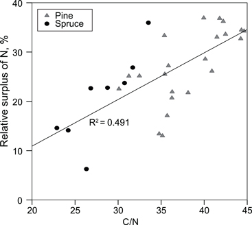
Fig. 3. Relative surplus of N in the organic layer, i.e. (amount of N on the fertilised plots – amount of N on the non-fertilised plots)/amount of N in fertilisers, as a function of the C/N ratio in the organic layer on the unfertilized plots.