Gintare Sabalinkiene  ,
Darius Danusevicius,
Michael Manton,
Gediminas Brazaitis,
Kastytis Simkevicius
,
Darius Danusevicius,
Michael Manton,
Gediminas Brazaitis,
Kastytis Simkevicius
Differentiation of European roe deer populations and ecotypes in Lithuania based on DNA markers, cranium and antler morphometry
Sabalinkiene G., Danusevicius D., Manton M., Brazaitis G., Simkevicius K. (2017). Differentiation of European roe deer populations and ecotypes in Lithuania based on DNA markers, cranium and antler morphometry. Silva Fennica vol. 51 no. 3 article id 1743. https://doi.org/10.14214/sf.1743
Highlights
- Lithuanian roe deer populations are genetically structured into southern and northern groups, most likely affected by a divergent gene flow and Lithuania’s largest rivers slowing down migration
- Microsatellite and skull morphology based genetic differentiation between field and forest ecotypes are weak
- Geographical location has a significant effect on antler morphometry traits and skull size of male roe deer, the latter increasing northwards.
Abstract
The objective of our study was to assess the genetic and morphological differentiation of European roe deer (Capreolus capreolus L.) in Lithuania based on DNA markers, skull and anther morphology. DNA was extracted from 79 culled individuals at 13 locations and genotyped at five nuclear microsatellite loci. Based on culling location, individuals were assigned to either a field (N = 43) or a forest ecotype (N = 36). Skull and antler morphometry was studied on 603 and 292 individuals, respectively. Results showed no significant genetic and skull morphology differentiation between the ecotypes. The forest ecotype tends to exhibit lower genetic diversity compared to the field ecotype, particularly for male individuals. The genetic differentiation of roe deer in Lithuania was significant based on the RST values, but not on the FST values. A STRUCTURE analyses revealed southern and northern genetic clusters, most likely affected by divergent gene flow. The country’s major rivers Nemunas and Neris are likely to increase differentiation between the clusters. ANOVA on skull morphology by gender and age indicated a significant effect of geographical location. Skull size (especially length) is greater in the northern part of the country. We also found significant effects of age, ecotype and geographical location on most of the roe deer male antler morphometric traits.
Keywords
genetic structure;
inbreeding;
Capreolus capreolus;
polymorphism;
wild game management
-
Sabalinkiene,
Institute of Forest Biology and Silviculture, Faculty of Forest Sciences and Ecology, Aleksandras Stulginskis University, Studentu street 11, Akademija, Kaunas district, Lithuania
E-mail
gintare.sabalinkiene@asu.lt
- Danusevicius, Institute of Forest Biology and Silviculture, Faculty of Forest Sciences and Ecology, Aleksandras Stulginskis University, Studentu street 11, Akademija, Kaunas district, Lithuania E-mail darius.danusevicius@asu.lt
- Manton, Institute of Forest Biology and Silviculture, Faculty of Forest Sciences and Ecology, Aleksandras Stulginskis University, Studentu street 11, Akademija, Kaunas district, Lithuania E-mail michael.manton@asu.lt
- Brazaitis, Institute of Forest Biology and Silviculture, Faculty of Forest Sciences and Ecology, Aleksandras Stulginskis University, Studentu street 11, Akademija, Kaunas district, Lithuania E-mail gediminas.brazaitis@asu.lt
- Simkevicius, Institute of Forest Biology and Silviculture, Faculty of Forest Sciences and Ecology, Aleksandras Stulginskis University, Studentu street 11, Akademija, Kaunas district, Lithuania E-mail kastytis.simkevicius@asu.lt
Received 12 December 2016 Accepted 23 May 2017 Published 9 June 2017
Views 139978
Available at https://doi.org/10.14214/sf.1743 | Download PDF

1 Introduction
Understanding the geographical distribution patterns of genetic and morphologic diversity constitutes the basis for sound management of game populations (Randi et al. 1998, 2004; Wang and Schreiber 2001). The effects of landscape structure, geographical features, urbanisation and game management intensity on both genetic structure and genetic diversity of European roe deer (Capreolus capreolus L.) populations are largely unknown in Lithuania. Understanding the effects of factors reducing gene flow, that leads to erosion of genetic variation is important (e.g. Kurt 1991). It is also important to assess how well skull and antler morphology reflects the genetic differentiation based on neutral DNA markers in roe deer.
Roe deer is a widespread wild mammal species in Europe. Through their ability to adapt to a broad range of environmental gradients, roe deer possess high levels of genetic diversity (Hartl et al. 1991, 1993). The genetic differentiation in roe deer is mainly affected by evolutionary history, social behaviour, hunting pressure, urbanization and environmental variation (e.g. Postma et al. 2001; Wang and Schreiber 2001; Brazaitis et al. 2014). Royo et al. (2007) revealed a significant differentiation between roe deer populations based on microsatellite markers in Spain. This differentiation was suggested to be caused by artificial introduction to enrich the historically overhunted populations, different post-glacial recolonization events, variable selective environments and natural mating barriers. Similarly, Fakler and Schreiber (1997) and Postma et al. (2001) reported significant microsatellite based differentiation between several roe deer populations in the Netherlands, where the country is small, the landscape is flat and no natural mating barriers exist. As in the Spanish study, the authors believe that the genetic differentiation in roe deer populations could have been caused by different ancestral histories. In Germany, Wang and Schreiber (2001) reported a homogeneous population that was not isolated by distance based on microsatellite markers. In Lithuania, genetic studies on roe deer are rare. Puraite et al. (2013) found phylogeny relationships separating the field and forest ecotypes of roe deer but observed no geographically interpretable patterns based on neutral DNA markers. In a comprehensive analysis of roe deer in southwestern France, Coulon et al. (2006) showed that highways, rivers and canals do not act as absolute barriers to movement, but they did produce subtle population differentiation. Intensive hunting may increase the heterozygosity by disrupting social groups in roe deer populations (Kurt 1991).
Regarding social behaviour, roe deer prefers forests opened by silviculture, but is also found in intensively cultivated agricultural land (Strandgaard 1972; Ellenberg 1978). Therefore, based on body size, behaviour and habitat, roe deer is often classified into the field or forest ecotypes (e.g. Raesfeld et al. 1985; Kurt 1991; Pėtelis and Brazaitis 2003). Stable social systems, such as matrilineal clans, are common in forests, where resource availability is more predictable and males maintain territories with several females and their offspring (Stubbe 1990; Kurt 1991). This strict family structure and limited migration may result in relatively higher level of inbreeding in the forest ecotype (Ellenberg 1978; Kurt et al. 1993). Whereas, unstable social structures prevail in field ecotypes, males rarely secure territories, family structure is hardly maintained, and females may copulate with several different males (Bresinski 1982; Kurt 1991). Males tend to disperse over larger distance than females, especially in the field ecotype (Ellenberg 1978; Stubbe 1990; Kurt 1991). On the other hand, the phenotype of roe deer is strongly affected by food resources, humidity, temperature, wind, population density, predators, diseases and parasites (Pélabon and Van Breukelen 1998; Vanpé et al. 2007). Morphological studies on roe deer in Lithuania and neighbouring countries indicate that body and cranium size are the most important indicators reflecting ecotype (Petelis and Brazaitis 2003). Roe deer of the field ecotype have adapted to breed in an open landscape where climate conditions are harsher due to lack of shelter, thus individuals are larger and heavier than individuals of the forest ecotype (Narauskaite and Petelis 2010). Studies of roe deer in southwestern Lithuania showed that their cranium continues to grow throughout life, and that roe deer of the field ecotype are significantly larger than those of the forest ecotype in the same region (Petelis and Brazaitis 2003). Indeed, Petelis and Brazaitis (2003) observed significant differences in cranium length, length of nasals and length of the tooth row in maxilla between the two ecotypes. Narauskaite et al. (2011) reported geographical differences in the body size of roe deer in Lithuania and identified the high importance of habitat quality, related to available food resources.
Studies of roe deer skull variation in western and central Europe (Aragon et al. 1998; Spencer 1995) shows that individuals with comparatively short and wide skulls feeds selectively on trees and shrubs throughout the year. In comparison, individuals with long skulls feed both on woody and herbaceous plants. These authors agree that the morphological differences among populations have environmental (phenotypic plasticity) rather than genetic origin. Labus et al. (2010) analysed roe deer sexual dimorphism by cranium morphometric traits and found significant variation only in 4 of 20 traits. They conclude that males have longer and wider skulls in comparison to females. The skulls of both males and females over the age of two, compared to those of younger individuals, are significantly different regarding most of the traits. Antler morphology is another socially and evolutionary important trait in roe deer. The European roe deer is a territorial animal (Bramley 1970), where males actively defend a territory, months ahead of the rut during July–August (Liberg et al. 1998). Territories are established in March–April and maintained over the summer, while in winter roe deer often form groups to feed in open habitat (Zejda 1978; San Jose et al. 1997). Territoriality of male roe deer mostly depends on the size of their antlers. Antlers may function as indicators of male strength and fighting ability in display toward other males. Females use this trait as a reliable signal of the sexual vigour when choosing the mates (Price et al. 1993; Wong and Candolin 2005). While several studies have shown a correlation between antler size or shape and body size (Pelabon and Van Breukelen 1998; Mysterud et al. 2005), unconditional dependence has rarely been comprehensively demonstrated.
The objectives of our study were two-fold, (1) to use DNA markers to assess the morphology variation, genetic structure and genetic diversity of geographical samples of roe deer, and (2) to use roe deer skull and antler morphometry to assess morphology and genetic differentiation between the forest and field ecotype in Lithuania.
2 Material and methods
2.1 DNA sampling
The muscle tissues from 79 culled roe deer individuals were collected at different geographical locations in Lithuania during the 2010–2012 hunting seasons and stored in a freezer at –70 °C (Table 1, Fig. 1). Hunting season for bucks (male roe deer) is from 15th May to 15th October and for doe and juveniles from 1st October to 31st December. During the hunting season, bucks are sessile, but may improve their home range in search for better food resources. The sex ratio was roughly equal with 43 females and 36 males. Individuals were grouped by ecotype – 43 individuals of field ecotype and 36 individuals of forest ecotypes were sampled. The ecotypes were identified based on the culling location. Roe deer of the field ecotype spend most of the year in open areas (Petelis and Brazaitis 2003). The culling location criteria for the field ecotype were: open land with < 20% forest cover within a 3 km radius from the culling site. Populations living in a large forested area or complex fragmented woods (e.g. forest cover > 20% within a 3 km radius of the culling site) were assigned as forest ecotype. We used eco-climatic zoning of the country (Karazija 1988) to test the regional effect on the morphology and genetic data. Not all populations used for morphometric analysis were used for DNA sampling.
| Table 1. The location of the populations (culling sites) and the number of sampled individuals for the DNA marker study. Population ID is given in numeric and letter format. Zone is eco-climatic zone (considered as region in the ANOVA). N is the number of individuals. Eco is the ecotype (Fo – forest ecotype population; Fld – field ecotype). | ||||||
| Pop id | Pop id | Zone | N | Eco | Latitude, Longitude | Culling location |
| ADE | 1 | I | 2 | Fo | 23°02´N, 55°48´E | Siauliai region, Kurtuvenu National Park, Naisiai |
| PLA | 2 | I | 3 | Fo | 21°53´N, 56°01´E | Plunge region, Plokstine forest |
| SIA | 3 | I | 3 | Fo | 23°22´N, 55°48´E | Siauliai region, Pakape forest |
| JON | 4 | II | 12 | Fld | 23°42´N, 56°16´E | Joniskis region |
| RAD | 5 | II | 8 | Fo | 23°29´N, 55°32´E | Radviliskis region, Bargailiai forest |
| NID | 6 | III | 4 | Fo | 21°01´N, 55°21´E | Neringa region, Briedziu forest |
| SIL | 7 | III | 9 | Fld | 21°21´N, 55°20´E | Silute region |
| ALY | 8 | IV | 3 | Fo | 23°58´N, 54°26´E | Alytus region |
| GIR | 9 | IV | 10 | Fo | 24°04´N, 54°49´E | Kaunas region, Dubrava forest |
| KAM | 10 | IV | 9 | Fld | 23°47´N, 54°54´E | Kaunas region, Kamsa forest |
| PRI | 12 | IV | 3 | Fo | 23°54´N, 54°36´E | Prienai region, Prienu Silas forest |
| VIR | 13 | IV | 13 | Fld | 22°48´N, 54°35´E | Vilkaviskis region, Virbalgiris forest and surrounding fields |
| Total | 79 | |||||
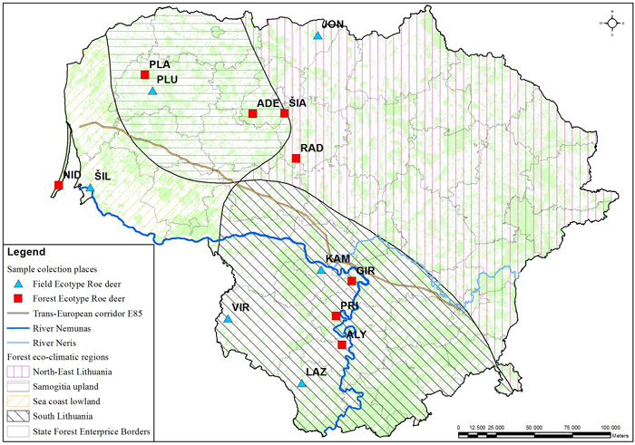
Fig. 1. Culling location of the sampled roe deer populations. The populations with field or forest ecotypes are indicated with different markers. Abbreviations explained in Table 1. The lines delineate the eco-climatic zones. The outlined populations were used for the DNA marker study. The populations marked in the map indicates the culling location. View larger in new window/tab.
2.2 DNA marker analysis
A muscle tissue sample of 10–30 mg was used for DNA-extraction by adding 180 μm Genomic Digestion Buffer and 20 μg Proteinase K. The solution was stored in a heating block for 3 hours at 55 °C, and centrifuged for 3 min at maximum speed. Then 20 μg of RNase A and 200 μg of Lysis Binding buffer were added, and vortexed. 200 μg of 70° ethanol was added to precipitate DNA. For DNA purification, the prepared lysate was added to a micro-tube and centrifuged at maximum speed. Washing buffer 1 was added to the micro-tube and centrifuged at maximum speed, repeating the procedure with washing buffer 2. After washing, 100 μg of the Elution buffer was added and centrifuged for 1 min at maximum speed. After checking the concentration, the DNA was stored in a freezer at –20 °C. Five nuclear microsatellite loci were used (Røed and Midthjell 1998; Postma et al. 2001; Lorenzini et al. 2004): NVHRT30, NVHRT71, NVHRT48, NVHRT16 and NVHRT24 (further abbreviated as N30, N71, N48, N16 and N24). We used two multiplex reactions for PCR amplification – N30 and N71 as multiplex No 1, and N48, N16 and N24 as multiplex No 2. The capillary electrophoresis was carried out with a genetic analyser (Applied Biosystems); allele sizing was performed using GeneMapper software (Applied Biosystems version 4.0).
The geographical differentiation among regions and populations was tested by the hierarchical AMOVA in GeneAlex v. 6.5 (Peakall and Smouse 2006) using the FST and RST fixation indexes (FST accounts for differentiation due to allele differences, while RST accounts for allele size differences among the entries). The total molecular variation was partitioned among regions, among populations within regions and within population, returning the following differentiation statistics: RST for combined population and region effect, RRT for region effect and RPT for population effect within region. The probability, P (rand > = data), for the fixation indexes was based on standard permutation across the full data set with 9999 permutations. The differentiation among ecotypes was tested with the FSTAT software using theta fixation index, which is less sample-size biased estimate of the Weir and Cockerham (1984) FST. The significance of the theta index was tested by calculating the standard error based on the jack knifing over loci and the 95% confidence interval by bootstrapping over loci, so that if these CI converges over zero the FST is considered not significantly different form zero. Rarefied allelic richness and inbreeding coefficient FIS were calculated with FSTAT software, after Weir and Cockerham (1984). The significance of the FIS index was tested by 200 randomizations, giving the proportion of the randomizations that gave smaller or larger value than the observed FIS value, indicating whether the FIS value is significantly negative or positive at the 5% significance level (significant excess or deficiency of heterozygotes).
Finally, we used the Bayesian clustering approach implemented in the software STRUCTURE ver. 2.1 (Pritchard et al. 2000) to estimate the most likely number of clusters (K) into which the microsatellite genotypes were assigned with certain likelihood. The population priors were not used. A Markov chain with 100 000 iterations following a burn-in period of 100 000 was used. Each run was replicated 10 times. The most likely number of clusters was identified by the delta K criterion with the STRUCTURE HARVESTER Web version 0.6.93 software (Earl and Holdt 2012). In addition, to decide the optimum number of clusters when the delta K value was not markedly different, we calculated the proportion of individuals with >0.7 likelihood for belonging to certain cluster and used it as a goodness-of-fit criterion. To assess the number of migrants per generation between the two STRUCTURE clusters, we (a) carried out AMOVA for differentiation between the two genetic groups identified by STRUCTURE, (b) used the formula for the number of migrants (Nm) by Clark and Hartl (1989): Nm = (1 / FST –1) / 4.
2.3 Skull and antler morphology traits
The roe deer skulls of 603 individuals (154 females and 449 males) from several geographical locations (coinciding with the culling locations sampled for the genetic analysis) were collected during the annual regional trophy evaluations in four eco-climatic zones in Lithuania: I – Samogitia upland (n = 26), II – Aukstaitija, northeastern Lithuania (n = 154), III – Seacoast lowland (n = 169) and IV – Suvalkija, southern Lithuania (n = 245) (Fig. 1). In each zone both forest and field ecotypes were sampled at nearly equal proportions. The culling location was considered to host a representative ecotype of roe deer population. Thus individuals were assigned into the ecotypes based on their living environment at the culling location. Using GIS, the state forest cadastre data from 2011 was used to evaluate the forest cover proportions in the living environment of each roe deer population. We sampled 238 individuals of the field ecotype and 365 individuals of the forest ecotype.
A set of 13 roe deer morphometric skull traits were measured with manual callipers (nearest 0.1 mm; based on Prusaite (1988); Narauskaite et al. (2011); shown in Fig. 2). Male and female skulls were divided into age classes according to Pélabon and Breukelen (1998): I age class (juvenile individuals from 6 up to 18 months); II age class (sub-adult individuals from 24 up to 36 months); III age class (individuals older than 36 months). The age of culled roe deer (males and females) was determined by the authors (the same persons for all individuals; educated and experienced as national trophy evaluation experts) based on milk tooth change to permanent, tooth attrition and skull joint ossification.
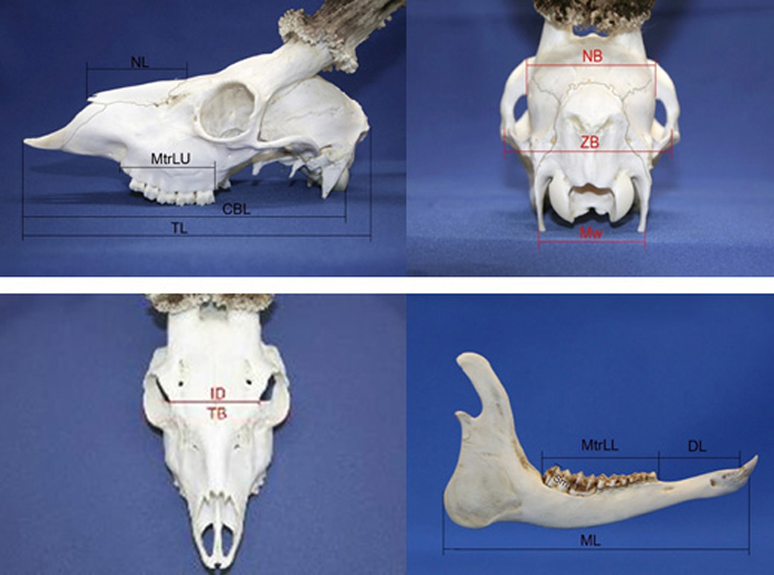
Fig. 2. Roe deer skull morphometry traits. View from the left side; NL – nasal length, MtrLU – maxilla tooth row length, CBL – condylobasal length, TL – total length of skull. View from the back side; NB – neurocranium breadth, ZB – zigomatic breadth, Mw – mastoidic width. View from the top; ID – interorbital distance, TB – total breadth. View from the right side of lower jaw; ML – Mandible length, MtrLL – mandible tooth raw length, DL – diastema length, Sm – the height of second molar tooth.
We measured antler morphometry of 292 male individuals as follows: I eco-climatic zone – 26 ind., II zone – 116 ind., III zone – 68 ind., IV zone – 82 individuals. 156 individuals were assigned as field ecotype and 136 individuals as forest ecotype. For comparative analysis we measured the length of right and left antler diameter, the circumstance of pedicles diameter, circumstance of roses, weight of antlers (together with a skull weight) and the span between antlers at the cranium at their biggest distance. The length of antler was measured to the nearest 0.1 cm along the external side of the main beam, from the base of antler to the top of main beam (Vanpé et al. 2007). The diameter and circumstance of pedicle were measured to the nearest 0.1 cm in the widest part of pedicle. The diameter and circumstance of both roses together were measured to the nearest 0.1 cm. The weight of antlers was measured to the nearest 1 g, together with the entire skull. The span between antlers was measured to the nearest 0.1 cm at the widest distance.
The 292 male individuals were grouped into five age classes according to development stage of antlers: age class 1 includes juvenile individuals up to 1.5 year, bearing first antler; age class 2 includes individuals from 1.5 to 2.5 years, bearing 2nd antlers; age class 3 includes individuals from 2.5 to 4.5 years, bearing 3rd and 4th antlers; age class 4 includes individuals from 4.5 to 5.5 years, bearing 5th antlers; and age class 5 includes individuals of 5.5 and older age.
We used ANOVA to compare roe deer skull and antler morphometric traits among regions, ecotypes, populations and age classes (PROC GLM in SAS software). The ANOVAs were run separately for each of the above given effects. To investigate the geographical variation patterns in the skull morphometry traits at the multivariate level, a Principal Component Analysis (PCA) was used at individual skull level as implemented in the PROC PRINCOMP in the SAS software.
3 Results
3.1 Genetic variation
All the microsatellite loci were polymorphic with 3 to 11 alleles, where N30 showed the lowest degree of polymorphism (Table 2). For N48 and N16, Ho was among the lowest and He among the highest (Table 2), indicating that the alleles are combined into homozygotes to a higher degree than in the remaining loci even if the alleles occur at relatively more equal frequencies (high Ne; He, Table 2). This increases the risk of inbreeding in future generations and is reflected by high positive values of the inbreeding coefficient FIS (Table 2). The loci N48 and N16 also showed significant population differentiation based on the FST index (Table 2). This implies that at loci N48 and N15, the roe deer populations are more fragmented with less gene-flow among them. Based on the RST fixation index, populations were significantly differentiated at all the loci, but at N48 and N16 the differentiation was stronger (Table 2).
| Table 2. The loci mean statistics (the standard error is given in the parenthesis, except for FST and RST for which the p values are given). The RST, FST differentiation is among roe deer populations. Na is total number of different alleles. Ne is the effective number of alleles He is expected heterozygosity (uHe is unbiased He corrected for sample size differences). FIS is inbreeding coefficient, RST and FST are the genetic differentiation indexes based on stepwise and infinitesimal mutation models. | |||||
| Index | N30 | N71 | N48 | N16 | N24 |
| Na | 3 | 9 | 7 | 11 | 11 |
| Ne | 2.01 (0.01) | 3.02 (0.31) | 3.70 (0.36) | 3.80 (0.50) | 2.60 (0.18) |
| Ho | 0.90 (0.05) | 0.73 (0.06) | 0.72 (0.07) | 0.64 (0.02) | 0.98 (0.02) |
| He | 0.50 (0.00) | 0.66 (0.03) | 0.72 (0.03) | 0.72 (0.03) | 0.61 (0.61) |
| uHe | 0.52 (0.00) | 0.68 (0.03) | 0.75 (0.04) | 0.75 (0.03) | 0.63 (0.03) |
| FIS | –0.79 (0.10) | –0.13 (0.13) | 0.01 (0.07) | 0.11 (0.06) | –0.62 (0.05) |
| RST | 0.051 (0.032) | 0.019 (0.153) | 0.088 (0.007) | 0.102 (0.004) | 0.068 (0.018) |
| FST | –0.019 (0.859) | –0.011 (0.778) | 0.032 (0.019) | 0.018 (0.057) | –0.007 (0.634) |
Gender had no effect on the genetic differentiation (the AMOVA p values for the fixation indexes were close to 1) and was ignored in further analysis of geographical differentiation based on the DNA markers. There was no marked difference between the sexes in multilocus genetic diversity indexes, except for the number of observed alleles being higher for females (5.8 and 7.0 alleles for males and females, respectively).
There was no significant genetic differentiation among the ecotypes (GeneAlex, FST = 0.001, p = 0.334; RST = 0.003, p = 0.265, Table 3). The locus-wise AMOVA for the ecotype effect based FST and RST indicated significant differentiation at the loci N30 and N71, respectively (Table 3). At the loci N48 and N16, the field ecotype was more genetically diverse possessing a lower inbreeding coefficient and higher observed heterozygosity than the forest ecotype (Fig. 3). The main differences in the genetic diversity index between the field and forest ecotypes were because of low genetic diversity of the males in the field ecotype (notable difference in Ho, Na and Ne, Table 4). The mean age of the forest and field males was similar of 3.80 and 3.52 years, respectively.
| Table 3. The differentiation indexes among the field and forest ecotypes based on AMOVA. | ||||||
| Index | N30 | N71 | N48 | N16 | N24 | Total |
| RST | 0.060 | –0.004 | –0.012 | –0.013 | –0.007 | 0.003 |
| p value (rand> = data) | 0.010 | 0.448 | 0.738 | 0.999 | 0.511 | 0.265 |
| FST | –0.005 | 0.027 | –0.002 | –0.007 | –0.009 | 0.001 |
| p value (rand> = data) | 0.462 | 0.028 | 0.483 | 0.803 | 0.859 | 0.334 |
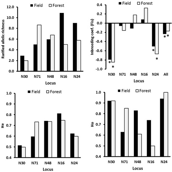
Fig. 3. The locus-wise genetic diversity parameters compared between the field and the forest ecotypes calculated with FSTAT software. For the inbreeding coefficient, the multilocus estimate was calculated (“all” on the X-axis, upper right plot). The asterisks mark the FIS values significant at the 0.05 level as estimated over 200 randomizations, based on the proportion of the randomizations that gave smaller or larger value than the observed value, so indicating significantly negative or positive FIS values.
| Table 4. Comparison of the multi loci genetic diversity parameters among the sexes within the field and forest ecotypes. N is the number of individuals. SE is standard error. The genetic diversity parameters are explained in Table 2. | ||||||||
| Ecotype/gender | Stat. | N | Na | Ne | Ho | He | uHe | FIS |
| Field/Female | Mean | 15.8 | 5.40 | 3.23 | 0.79 | 0.64 | 0.66 | –0.30 |
| SE | 1.20 | 0.68 | 0.06 | 0.05 | 0.06 | 0.18 | ||
| Forest/Female | Mean | 24.8 | 5.40 | 3.13 | 0.79 | 0.65 | 0.67 | –0.26 |
| SE | 1.10 | 0.37 | 0.07 | 0.04 | 0.04 | 0.20 | ||
| Field/Male | Mean | 20.2 | 5.20 | 3.09 | 0.82 | 0.65 | 0.66 | –0.29 |
| SE | 1.10 | 0.40 | 0.07 | 0.04 | 0.04 | 0.15 | ||
| Forest/Male | Mean | 13.6 | 4.20 | 2.89 | 0.72 | 0.63 | 0.65 | –0.22 |
| SE | 0.70 | 0.33 | 0.13 | 0.04 | 0.04 | 0.28 | ||
Because there was no significant differentiation between ecotypes, we analysed the geographical differentiation by ignoring ecotypes. The RST-based AMOVA revealed a significant eco-climatic zone effect (RST = 0.092, p = 0.008; RRT = 0.101, p = 0.003) and no significant population effect within zone (RPT = 0). The percentages of variation among the zones, among the populations within region and within populations were 10%, 0%, 90%, respectively. In the FST based AMOVA, the zone differentiation was not significant (FST = 0.010, p = 0.201; FRT = 0.006, p = 0.299; FPT = 0.003, p = 0.386).
For the within population genetic diversity comparison, we ignored the populations with a sample size less than 4. The mean number of alleles varied from 3.0 in Girionys (GIR) (a suburb of a large city) to 4.8 in Joniskis (JON) and Virbalgiris (VIR) populations (Table 5). The FIS values for all populations were negative indicating no marked excess of homozygotes (Fig. 4). The Nida (NID) population located on the sea-side spit of Neringa (Fig. 1) possessed the highest FIS value, indicating a relatively greater proportion of homozygotes (Fig. 4). A similar situation with a relatively higher FIS index was found within the Girionys (GIR) and Kamsa (KAM) populations, both locations are suburbs of Kaunas, Lithuania’s second biggest city and adjacent to the large water bodies of the Nemunas river and Kauno Marios lagoon, which also seems to have an effect on reducing migration possibilities.
| Table 5. The multilocus mean within population (culling location) genetic diversity indexes. The eco-climatic zone is given in the parenthesis at the population name. N is the number of individuals. Data for populations with sample size > = 4 are shown. | ||||||
| Pop (eco climatic zone) | N | Na | Ne | Ho | uHe | FIS |
| JON (2) | 12 | 4.80 | 3.00 | 0.80 | 0.67 | –0.27 |
| RAD (2) | 8 | 3.80 | 3.03 | 0.90 | 0.69 | –0.44 |
| NID (3) | 4 | 3.40 | 2.77 | 0.73 | 0.71 | –0.20 |
| SIL (3) | 9 | 3.60 | 2.72 | 0.78 | 0.65 | –0.33 |
| GIR (4) | 10 | 3.00 | 2.54 | 0.69 | 0.63 | –0.23 |
| KAM (4) | 10 | 4.00 | 2.53 | 0.71 | 0.61 | –0.24 |
| PRI (4) | 12 | 2.80 | 2.31 | 0.73 | 0.67 | –0.35 |
| VIR (4) | 13 | 4.80 | 3.33 | 0.87 | 0.69 | –0.36 |
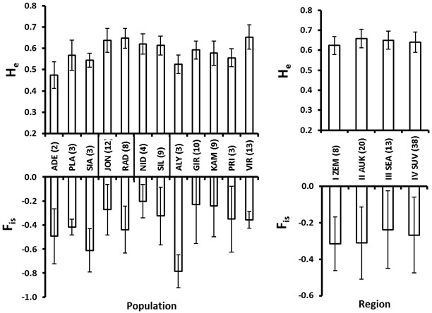
Fig. 4. Roe deer culling location (population, left) and eco-climatic zone (region, right) mean and standard error values for expected heterozygosity (He) and the inbreeding coefficient (FIS). Number of individuals in each population and region is given in the parenthesis at the abbreviations of the populations (culling locations), which are explained in Table 2. The vertical lines at the X-axis in the left plot delineate regions (eco-climatic zones).
The Bayesian clustering in the STRUCTURE analysis revealed the highest likelihood of two genetically distinct clusters in Lithuania (Fig. 5). The Delta K value and the proportion of populations with >0.7 likelihood of belonging to a genetic cluster were the greatest for the structure with two genetic clusters (not shown). Based on the relative shares of the two STRUCTURE clusters, geographically two genetically distinct groups can be distinguished in Lithuania: (a) the northern group, located north of the country’s main rivers Nemunas and Neris; populations 1 to 7 (Fig. 5), where the STRUCTURE cluster 1 (separated by STRUCTURE) was dominant; and (b) the southern group, populations 8 to 13, where the STRUCTURE cluster 2 was dominant (Fig. 5). However, none of the populations studied were fixed to a specific STRUCTURE cluster (Fig. 5).
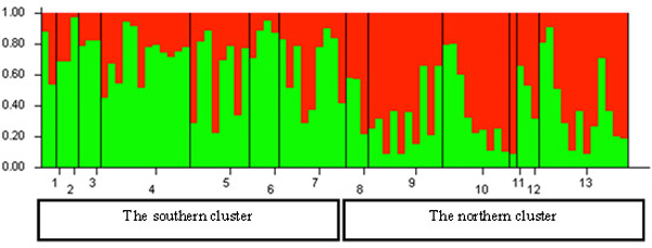
Fig. 5. Histogram of genetic structure of roe deer in Lithuania based on Bayesian clustering with STRUCTURE software. The two colours represent different STRUCTURE clusters. Populations are separated by vertical lines and identified on the X-axis by numbers (pop id in Table 1), where larger sample sizes correspond to longer intervals on the X-axis (each individual is a separate colour line). Y-axis is the likelihood for the individual membership into each of the two clusters separated by the STRUCTURE software and indicated here with different colour. The southern cluster includes individuals sampled in southern Lithuania and seacost lowland eco-climatic zones. The northern cluster includes individuals sampled in northeastern Lithuania and Samogitia upland.
By containing the highest proportion of the individuals ascribed to cluster 1, the Nida population No. 6 located on the sea-side spit was the most divergent from the other populations in the northern group (Fig. 5). Whereas, the population of Silute (SIL) (No. 7) possessed a greater proportion of the cluster 2 genotypes than the Nida population which is located on the opposite of the Kursiu Marios lagoon (Fig. 5).
3.2 Skull morphology variation
The mean skull length increased with age from 18.2 cm at age class 1 (0–1 years) to 20.4 cm at age class 3 (age 3–10 years), with the minimum value of 16.2 cm at the 1st age class and maximum value of 22.3 cm at the 3rd age class. The total skull breadth increased from 8.1 cm at the 1st age class to 9.3 cm at the 3rd age class. The mean values of all the measured traits increased with age (Table 6). This indicates that skull size continues to increase within all three age classes. The mean height of second molar decreased with the age. The greatest skull increment from the 1st to the 3rd age classes was observed in following traits: diastema length, nasal length, mandible tooth raw length, total breadth, 15.9%, 15.3%, 13.8% and 12.9% respectively, indicating a greater growing potential of the frontal zone of the skull. Whereas, neurocranium length and mastoidic width increased from the 1st to 3rd age classes only 6.6% and 6.5%, respectively.
| Table 6. The mean value and the variance of roe deer skull morphology traits, given by three age classes. Age class 1st (age from 0 to 1 years), age class 2 (age from 2 years to 3 years), age class 3 (age from 3 years to 10 years). M is a mean value, N is the number of individuals, CV is a coefficient of variance, Min and Max is a minimal and maximal values. The abbreviations of the traits are explained in Fig. 2. | |||||||||||||||
| Variable | AGE CLASS = 1 | AGE CLASS = 2 | AGE CLASS = 3 | ||||||||||||
| M | N | CV | Min | Max | M | N | CV | Min | Max | M | N | CV | Min | Max | |
| TLENGHT | 18.2 | 110 | 4.9 | 16.2 | 20.9 | 19.8 | 32 | 3.2 | 18.6 | 21.0 | 20.4 | 388 | 3.4 | 18.6 | 22.3 |
| CLENGHT | 17.1 | 110 | 4.8 | 15.4 | 19.6 | 18.7 | 32 | 3.7 | 17.5 | 20.0 | 19.3 | 385 | 3.4 | 17.5 | 21.2 |
| TBREADTH | 8.1 | 118 | 5.1 | 7.2 | 9.0 | 8.9 | 40 | 3.7 | 8.2 | 9.6 | 9.3 | 445 | 4.7 | 7.8 | 10.6 |
| ORBDIST | 4.9 | 118 | 8.5 | 4.3 | 7.2 | 5.3 | 40 | 6.5 | 4.6 | 6.7 | 5.5 | 445 | 6.5 | 4.5 | 6.9 |
| ZBREADTH | 6.5 | 116 | 9.9 | 4.9 | 8.2 | 7.2 | 40 | 7.7 | 6.3 | 8.8 | 7.4 | 443 | 8.5 | 5.2 | 9.0 |
| NASALONG | 5.0 | 108 | 9.0 | 3.9 | 7.0 | 5.8 | 39 | 7.2 | 5.0 | 6.6 | 5.9 | 432 | 8.4 | 4.5 | 7.2 |
| NEURLONG | 5.7 | 117 | 3.6 | 5.3 | 6.2 | 5.9 | 40 | 3.6 | 5.4 | 6.4 | 6.1 | 442 | 3.8 | 5.4 | 6.7 |
| MTOOTR | 5.2 | 108 | 7.1 | 4.4 | 6.3 | 5.9 | 34 | 4.7 | 5.1 | 6.4 | 5.7 | 353 | 4.4 | 5.1 | 6.5 |
| MATOOTR | 5.6 | 114 | 10.1 | 4.5 | 7.0 | 6.6 | 39 | 4.5 | 6.1 | 7.2 | 6.5 | 361 | 4.3 | 3.9 | 7.4 |
| DIASTEM | 3.7 | 113 | 7.6 | 3.0 | 4.5 | 4.1 | 39 | 7.7 | 3.4 | 5.2 | 4.4 | 414 | 7.7 | 3.2 | 5.6 |
| MANDIBL | 14.2 | 113 | 5.6 | 12.4 | 16.3 | 15.5 | 38 | 3.7 | 14.6 | 16.8 | 16.0 | 395 | 3.5 | 13.7 | 17.2 |
| MASTOTIC | 4.3 | 89 | 6.7 | 3.6 | 5.0 | 4.5 | 35 | 8.7 | 3.7 | 6.1 | 4.6 | 263 | 8.0 | 3.7 | 5.7 |
| M2H | 0.7 | 70 | 16.4 | 0.4 | 0.8 | 0.7 | 35 | 10.4 | 0.5 | 0.9 | 0.6 | 340 | 19.4 | 0.2 | 0.9 |
| Trait abbreviations (see also Fig. 2); TBREADTH is total skull breadth, CLENGHT is total skull length, ORBDIST is interorbital distance, ZBREADTH is zigomatic breadth, NASALONG is nasal length, NEURLONG is a neurocranium length, MTOOTR is a maxilla tooth row length, MATOOTR is a mandible tooth row length, DIASREM is a diastema length, | |||||||||||||||
There was a relatively stronger effect of gender on the skull morphology traits at the juvenile age (Table 7). For zygomatic breadth, the effect of gender was equally important in all age classes, whereas for mandible length, maxilla and mandible tooth raw length, length of nasals, the gender effect was stronger at the juvenile stage than at the mature stage (Table 7). For diastema length, mastoidic width, age had a relatively stronger effect at the mature stage. The males showed higher measurement values in almost all measured traits in all age classes (Table 7).
| Table 7. The results of ANOVA on the effect of the eco-climatic zone on roe deer skull morphometry run separately for male and female individuals and age class. DF for error by age class 1, 2, 3 (males) = 55, 31, 351; DF for error female = 55; 3; 85. F is the Fisher’s criterion and p > F is the significance of F from the ANOVA. The abbreviations of the traits are explained in Fig. 2. Bold values indicates a significant variance in particular traits and age classes. | ||||||
| AGE CLASS | NAME | DF | Males | Females | ||
| F | p > F | F | p > F | |||
| 1 | TLENGHT | 3 | 2.7 | 0.0575 | 1.8 | 0.1665 |
| 2 | TLENGHT | 3 | 0.5 | 0.6824 | 0.2 | 0.7172 |
| 3 | TLENGHT | 3 | 3.4 | 0.0189 | 0.3 | 0.8042 |
| 1 | CLENGHT | 3 | 2.9 | 0.0455 | 2.5 | 0.0707 |
| 2 | CLENGHT | 3 | 0.8 | 0.4982 | 1.0 | 0.3895 |
| 3 | CLENGHT | 3 | 5.2 | 0.0016 | 0.0 | 0.9908 |
| 1 | TBREADTH | 3 | 2.9 | 0.0409 | 1.6 | 0.1965 |
| 2 | TBREADTH | 3 | 1.9 | 0.1586 | 2.8 | 0.1926 |
| 3 | TBREADTH | 3 | 1.3 | 0.2835 | 0.6 | 0.6415 |
| 1 | ORBDIST | 3 | 1.4 | 0.2645 | 1.4 | 0.2389 |
| 2 | ORBDIST | 3 | 0.9 | 0.4525 | 2.0 | 0.2530 |
| 3 | ORBDIST | 3 | 0.5 | 0.6953 | 0.2 | 0.8741 |
| 1 | ZBREADTH | 3 | 2.7 | 0.0540 | 0.2 | 0.8817 |
| 2 | ZBREADTH | 3 | 0.1 | 0.9371 | 1.0 | 0.3937 |
| 3 | ZBREADTH | 3 | 6.5 | 0.0003 | 2.9 | 0.0418 |
| 1 | NASALONG | 3 | 4.3 | 0.0087 | 0.1 | 0.9383 |
| 2 | NASALONG | 3 | 1.2 | 0.3175 | 4.0 | 0.1397 |
| 3 | NASALONG | 3 | 0.9 | 0.4467 | 0.1 | 0.9424 |
| 1 | NEURLONG | 3 | 0.3 | 0.8008 | 2.5 | 0.0711 |
| 2 | NEURLONG | 3 | 1.0 | 0.4208 | 1.3 | 0.3357 |
| 3 | NEURLONG | 3 | 2.9 | 0.0342 | 0.9 | 0.4503 |
| 1 | MTOOTR | 3 | 2.5 | 0.0721 | 5.3 | 0.0029 |
| 2 | MTOOTR | 3 | 1.6 | 0.2168 | 0.6 | 0.4912 |
| 3 | MTOOTR | 3 | 9.5 | 0.0000 | 0.1 | 0.9839 |
| 1 | MATOOTR | 3 | 9.9 | 0.0000 | 1.8 | 0.1555 |
| 2 | MATOOTR | 3 | 1.6 | 0.2002 | 0.3 | 0.6134 |
| 3 | MATOOTR | 3 | 2.9 | 0.0345 | 5.2 | 0.0025 |
| 1 | DIASTEM | 3 | 4.8 | 0.0052 | 0.5 | 0.7178 |
| 2 | DIASTEM | 3 | 1.0 | 0.4016 | 2.8 | 0.1938 |
| 3 | DIASTEM | 3 | 19.1 | 0.0000 | 0.4 | 0.7203 |
| 1 | MANDIBL | 3 | 6.5 | 0.0008 | 1.7 | 0.1879 |
| 2 | MANDIBL | 3 | 0.7 | 0.5563 | 0.2 | 0.6737 |
| 3 | MANDIBL | 3 | 0.6 | 0.6263 | 0.4 | 0.7831 |
| 1 | MASTOTIC | 3 | 0.7 | 0.5426 | 0.4 | 0.7789 |
| 2 | MASTOTIC | 3 | 0.1 | 0.9565 | 0.1 | 0.8074 |
| 3 | MASTOTIC | 3 | 0.2 | 0.8903 | 1.2 | 0.3002 |
| 1 | M2H | 3 | 0.5 | 0.6877 | 1.2 | 0.3326 |
| 2 | M2H | 3 | 2.3 | 0.1061 | 0.0 | 0.9205 |
| 3 | M2H | 3 | 2.1 | 0.0966 | 1.2 | 0.3112 |
The ANOVA for male revealed a stronger regional effect than for females in most of the skull morphology traits (Table 7). Furthermore, we observed a significant regional effect on skull size in particular age classes (Table 7). At a mature age (e.g., age class 5), male individuals from northern Lithuania possessed significantly larger skulls (both breath and width) than from southern Lithuania. Whereas, the female skull length varied little between the regions, however, there was a tendency of smaller skulls in the southern Lithuania (Table 7).
Owing to the significant effect of sex and age on the skull morphological traits studied (the ANOVAs above) we carried out a separate principal component analysis for each gender and age class. The principal component analysis revealed that the first pair of principal components (PCs) explains 60–70% and 50–60% the variation of the skull morphology traits for male and for female individuals, respectively. For male individuals at age class 3, the plot of individual PC scores against the first pair of the PCs, revealed possible clusters of individuals based on the geographical location (Fig. 6). There was a tendency for individuals from the eco-climatic zones I and II (northeastern Lithuania and Samogitia upland to possess higher scores for the PC1 (Fig. 6.). This indicates larger skulls and the associated skull size variables in northern Lithuania than in the southern Lithuania.
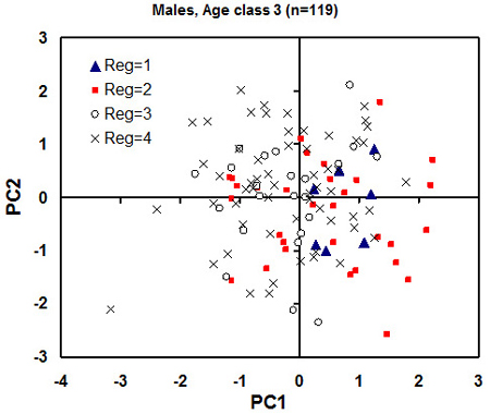
Fig. 6. Plot of individual principal component (PC) scores against the first pair of the PC from the principal component analysis for the male individuals of age class 3 (adults). Each eco-climatic zone (“Reg” on the plot) is marked with different markers. 1 is Samogitia upland, 2 is northeastern Lithuania, 3 is seaside lowland, 4 is southern Lithuania. The regional mean standard error for PC1 and PC2 scores is 1.5 and 2.0, respectively (to be used as an estimate of least significant difference). A tendency for higher PC1 scores of the northern regions 1 and 2 (meaning greater skull dimensions) is observed.
When running the ANOVAS on the ecotype effect by the age classes with the gender pooled, our results revealed no significant ecotype effect for most of the skull morphology traits (Table 8). The significant difference between the ecotypes was found in zygomatic breadth of skull at age class 2, maxilla tooth raw length at age class 2 and diastema length in at age class 3 (Table 8).
| Table 8. Results of ANOVA on the ecotype effect run separately for each age class. N is the number of roe deer individuals, SE is the standard error. F is the Fisher’s criterion and p is the significance of F from the ANOVA. The abbreviations of the variables are explained in Fig 2. Bold values indicates a significant variance in particular traits and age classes. | |||||||||
| Age class | Variable | ECOTYPE = Field | ECOTYPE = Forest | F | p > F | ||||
| Mean | N | SE | Mean | N | SE | ||||
| 1 | TLENGHT | 18.3 | 41 | 0.16 | 18.1 | 69 | 0.10 | 1.2 | 0.2813 |
| 2 | TLENGHT | 19.7 | 19 | 0.15 | 19.9 | 13 | 0.17 | 0.5 | 0.4744 |
| 3 | TLENGHT | 20.5 | 154 | 0.06 | 20.4 | 234 | 0.04 | 1.2 | 0.2675 |
| 1 | CLENGHT | 17.2 | 41 | 0.15 | 17.1 | 69 | 0.09 | 0.8 | 0.3631 |
| 2 | CLENGHT | 18.5 | 19 | 0.16 | 18.9 | 13 | 0.18 | 2.1 | 0.1586 |
| 3 | CLENGHT | 19.3 | 154 | 0.06 | 19.2 | 231 | 0.04 | 1.2 | 0.2814 |
| 1 | TBREADTH | 8.1 | 42 | 0.07 | 8.1 | 76 | 0.04 | 0.0 | 0.9134 |
| 2 | TBREADTH | 8.9 | 23 | 0.08 | 8.8 | 17 | 0.07 | 0.5 | 0.4829 |
| 3 | TBREADTH | 9.3 | 173 | 0.03 | 9.3 | 272 | 0.03 | 0.0 | 0.8798 |
| 1 | ORBDIST | 4.8 | 42 | 0.05 | 4.9 | 76 | 0.05 | 3.1 | 0.0804 |
| 2 | ORBDIST | 5.3 | 23 | 0.05 | 5.3 | 17 | 0.11 | 0.0 | 0.9958 |
| 3 | ORBDIST | 5.5 | 173 | 0.03 | 5.5 | 272 | 0.02 | 1.3 | 0.2552 |
| 1 | ZBREADTH | 6.5 | 42 | 0.12 | 6.5 | 74 | 0.07 | 0.0 | 0.8367 |
| 2 | ZBREADTH | 7.4 | 23 | 0.12 | 7.0 | 17 | 0.10 | 7.1 | 0.0110 |
| 3 | ZBREADTH | 7.4 | 172 | 0.05 | 7.4 | 271 | 0.04 | 0.1 | 0.7841 |
| 1 | NASALONG | 5.0 | 40 | 0.07 | 5.0 | 68 | 0.06 | 0.2 | 0.6909 |
| 2 | NASALONG | 5.8 | 23 | 0.09 | 5.8 | 16 | 0.11 | 0.0 | 0.9381 |
| 3 | NASALONG | 5.9 | 166 | 0.04 | 5.9 | 266 | 0.03 | 0.5 | 0.4674 |
| 1 | NEURLONG | 5.7 | 42 | 0.03 | 5.7 | 75 | 0.02 | 0.0 | 0.9298 |
| 2 | NEURLONG | 5.9 | 23 | 0.04 | 6.0 | 17 | 0.05 | 0.2 | 0.6366 |
| 3 | NEURLONG | 6.1 | 173 | 0.02 | 6.1 | 269 | 0.01 | 0.6 | 0.4456 |
| 1 | MTOOTR | 5.3 | 41 | 0.08 | 5.2 | 67 | 0.03 | 1.3 | 0.2547 |
| 2 | MTOOTR | 5.9 | 23 | 0.05 | 5.7 | 11 | 0.08 | 5.0 | 0.0331 |
| 3 | MTOOTR | 5.7 | 170 | 0.02 | 5.7 | 183 | 0.02 | 2.5 | 0.1163 |
| 1 | MATOOTR | 5.7 | 40 | 0.10 | 5.6 | 74 | 0.06 | 0.6 | 0.4413 |
| 2 | MATOOTR | 6.6 | 22 | 0.06 | 6.5 | 17 | 0.08 | 1.0 | 0.3304 |
| 3 | MATOOTR | 6.5 | 150 | 0.02 | 6.5 | 211 | 0.02 | 0.9 | 0.3336 |
| 1 | DIASTEM | 3.8 | 41 | 0.04 | 3.7 | 72 | 0.03 | 2.5 | 0.1148 |
| 2 | DIASTEM | 4.0 | 22 | 0.07 | 4.2 | 17 | 0.07 | 3.0 | 0.0919 |
| 3 | DIASTEM | 4.3 | 164 | 0.02 | 4.4 | 250 | 0.02 | 4.6 | 0.0328 |
| 1 | MANDIBL | 14.2 | 41 | 0.14 | 14.1 | 72 | 0.09 | 0.2 | 0.6535 |
| 2 | MANDIBL | 15.3 | 21 | 0.13 | 15.6 | 17 | 0.12 | 2.3 | 0.1394 |
| 3 | MANDIBL | 16.0 | 162 | 0.04 | 16.0 | 233 | 0.04 | 0.1 | 0.8139 |
| 1 | MASTOTIC | 4.2 | 32 | 0.04 | 4.3 | 57 | 0.04 | 3.4 | 0.0672 |
| 2 | MASTOTIC | 4.6 | 21 | 0.09 | 4.4 | 14 | 0.09 | 1.6 | 0.2179 |
| 3 | MASTOTIC | 4.7 | 125 | 0.03 | 4.6 | 138 | 0.03 | 2.9 | 0.0907 |
| 1 | M2H | 0.6 | 28 | 0.02 | 0.7 | 42 | 0.01 | 0.6 | 0.4427 |
| 2 | M2H | 0.7 | 19 | 0.02 | 0.7 | 16 | 0.02 | 0.0 | 0.9472 |
| 3 | M2H | 0.6 | 134 | 0.01 | 0.6 | 206 | 0.01 | 0.0 | 0.9703 |
3.3 Variation in male roe deer antler morphology
All the measured traits of male roe deer antlers were significantly different among all age classes (Table 9). As expected, antlers increased in size with age, the highest values were recorded in age class 5. The main roe deer antler morphometric traits, e.g. length and weight of antlers, recorded the highest mean values at age class 4, followed by a decrease at age class 5. The pedicle and the roses of antler are continuously increasing and widening over the life span of an individual, including age class 5. The span between the antlers peaked in age class 4.
| Table 9. The comparison of male roe deer antler traits among the age classes. F is the ANOVA Fisher’s criterion and p is the significance of F from the ANOVA with age as class the independent variable. SE is standard error. | |||||||||
| Age class (number of individuals) | Length of right buck, cm | Length of left buck, cm | Diameter of pedicle, cm | Circumstance of pedicle, cm | Circumstance of roses, cm | Diameter of roses, cm | Weight, g | Span between bucks, cm | |
| F | 38.4 | 37.5 | 28.0 | 29.9 | 15.9 | 25.9 | 28.6 | 10.7 | |
| p > F | 0.0001 | <0.0001 | <0.0001 | <0.0001 | <0.0001 | <0.0001 | <0.0001 | <0.0001 | |
| Age class 1 n = 15 | Mean | 11.81 | 11.99 | 1.50 | 4.82 | 13.30 | 5.06 | 186.72 | 5.20 |
| SE | 1.0 | 1.0 | 0.1 | 0.2 | 1.1 | 0.4 | 21.5 | 0.9 | |
| Age class 2 n = 32 | Mean | 14.41 | 14.56 | 1.71 | 5.42 | 15.32 | 5.76 | 255.76 | 7.54 |
| SE | 0.7 | 0.7 | 0.06 | 0.2 | 0.8 | 0.2 | 14.8 | 0.6 | |
| Age class 3 n = 83 | Mean | 18.57 | 18.52 | 1.90 | 6.01 | 15.90 | 6.44 | 294.91 | 8.56 |
| SE | 0.4 | 0.4 | 0.03 | 0.1 | 0.4 | 0.1 | 8.5 | 0.4 | |
| Age class 4 n = 52 | Mean | 21.57 | 21.68 | 2.15 | 6.86 | 19.09 | 7.34 | 365.60 | 10.05 |
| SE | 0.6 | 0.6 | 0.04 | 0.1 | 0.6 | 0.2 | 10.3 | 0.5 | |
| Age class 5 n = 110 | Mean | 21.45 | 21.59 | 2.23 | 6.96 | 19.28 | 7.76 | 357.3 | 10.10 |
| SE | 0.4 | 0.4 | 0.0 | 0.1 | 0.4 | 0.1 | 7.5 | 0.3 | |
The ANOVA revealed significant regional effect on the antler morphometric traits of roe deer (not shown). Such traits as the length of antlers (right, p = 0.0001; left, p < 0.0001), diameter (p = 0.0025) and circumstance (p = 0.0002) of pedicle, diameter (p < 0.0001) and circumstance (p = 0.0002) of roses, antler weight (p = 0.0009) and the span between antlers (p = 0.0383) were significantly different among the eco-climatic regions. In the pooled over all age classes ANOVA, the ecotype had a significant effect on the following traits: the length of antlers (p = 0.0037; p = 0.0002, right and left antler, respectively) the diameter of pedicle (p = 0.0449), the diameter of roses (p = 0.0700), the weight (p = 0.0572) and the span between antlers (p = 0.0273). However, the circumstance of pedicle and the circumstance of roses were not significantly different among the ecotypes.
The comparison of roe deer antler morphometric measurement traits among the populations showed significant differences in all measured traits: the length of right antler (p = 0.0024), length of left antler (p = 0.0004), diameter of pedicle (p = 0.0031), circumstance of pedicle (p < 0.0001), circumstance of roses (p = 0.0019), diameter of roses (p < 0.0001), weight of antlers (p = 0.0020) and span between antlers (p = 0.0057).
4 Discussion
4.1 Age effect on the morphometric variation
In agreement with Petelis and Brazaitis (2003), we found that the cranium of roe deer is continuously growing throughout its life. The highest rate of skull growth was observed at a young age – first and second age classes. The growth increment of roe deer skulls is reduced after 4–5 year of age (not shown). In roe deer, antler morphology can provide information about the age (Strandgaard 1972) and potential quality (Wahlström 1994). The size and shape of antlers are age dependent and have typical development stages within different age classes (Baleisis et al. 2003). Our results on the age effect confirm that the roe deer reach their trophic maturity during the 4th age class (fifth antler). However, there were also large individual differences in antler size and shape within the given age classes. Therefore, antler size is generally considered as an unreliable indicator of age (e.g. Prior 2000).
4.2 Gender effect on genetic and morphometric variation
We found no genetic differentiation among sexes at the neutral microsatellite loci. However, gender had a significant effect on roe deer skull size and shape, especially at the frontal zone of the skull. This can be contributed to the annual growing and shedding of antlers by males. Males had a significantly wider skull, wider interorbital distance, and longer frontal zone. Indeed the differences in body and skull size between the sexes and among age classes are well recognized in roe deer (Petelis and Brazaitis 2003; Labus et al. 2010). We observed a large difference in skull size among the sexes at the juvenile age, when the skull size is still developing. The difference in scull size between sexes is largely affected by vegetation type and structure of habitat (Perez-Barberia et al. 2002).
4.3 Ecotype effect on genetic and morphometric variation
In contrary to what had been expected, the study of skull morphometric traits variation among forest and field ecotype individuals showed no significant effect of ecotype in roe deer in the ANOVA for the overall dataset. Most likely the lack of natural mating barriers and small scale landscape fragmentation, allows gene flow among the field and forest ecotypes. We presume that during the 1960–70’s the roe deer population split into the two current ecotype populations (field and forest) as a response to a high density of cervids, the introduction of fallow deer (Cervus dama L.) and the industrialisation of agriculture. Intensification of silviculture and agriculture drastically changed the Lithuanian landscape. These developments and factors pushed the roe deer out of forests into the open landscape. However, these events were recent and could not have solely caused genetic differentiation. Thus the field and forest ecotype of roe deer actually extends further back in time. In Austria, Kurt et al. (1993) found no genetic differentiation between roe deer in forest and field ecotypes, but found the level of inbreeding significantly high (high FIS value) in the forest ecotype based on allozymes. Interestingly, Kurt et al. (1993) also found that after including the populations with high culling rates, the FIS became significantly negative for the forest ecotype, indicating that hunting may disturb the social structure and increase the heterozygosity. In contrast, Puraite et al. (2013) reported a dendrogram based clustering into field and forest ecotype clades based on RAPD (randomly amplified polymorphic DNA) markers in Lithuania.
A lower genetic diversity of the forest ecotype in our study suggests a tendency of stricter herd structure, stable male-female relationships in the forest ecotype with fewer migrants, causing relatively more frequent mating among relatives and higher inbreeding than for the field ecotype, which is supported by Strandgaard 1972, Ellenberg 1978 and Kurt et al. (1993). In our study, the main differences in genetic diversity between the ecotypes were mainly at the cost of low diversity of the field ecotype males. This supports the migration related cause of the low genetic diversity in the forest ecotype (Table 4). Namely males tend to migrate over larger distances than females and are believed to be a strong source of gene flow in roe deer (Ellenberg 1978; Stubbe 1990; Kurt 1991). This observation corresponds well to the social behaviour of roe deer with a strong family clan structure of the forest ecotype in contrast to the field ecotype roe deer dwelling in open agricultural landscape (Bresinski 1982). The migration distances of the field ecotype are presumably larger than of the forest ecotype, with the latter often limited to their own forest tracts (Danilken and Hewison 1996). Thus the possibility for mating with more distant and genetically different individuals is greater for the field roe deer ecotype compared to roe deer of the forest ecotype.
In our study, the individuals of the forest ecotype were sampled after culling in intensively hunted areas. Hunting may have a positive effect on genetic diversity by interfering with the strict family and territorial structure and thus contribute to inter clan mating (Kurt 1991). The clan structure and the diversifying effects of hunting counteract each other and may lead to similar results as in our study with slightly lower diversity for males in the forest ecotype.
4.4 Geographic location effect on the genetic and morphometric variation
In agreement with the microsatellite-based studies on roe deer in central Europe (e.g. Postma et al. 2001; Wang and Sriebel 2001), we found high levels of polymorphism at all the loci investigated. The geographical effect on genetic differentiation was not strong in Lithuania, indicating extensive gene-flow between the populations. The remaining differentiation may be due to recent (post-glacial) population development and evolutionary background. Divergent migration together with mutations may result in similar levels of differentiation as observed in our study. Populations in northeastern Lithuania may receive genetically differing migrants (Russia) than populations in southern Lithuania (Poland). In support, we observed population-specific alleles in the Samogitia upland region (Fig. 4). Our observation of stronger RST than FST based differentiation indicates the importance of the stepwise mutation model for population differentiation, indicating that this is an evolutionary younger differentiation than the post-glacial lines. In a microsatellite based study of roe deer in Germany, Wang and Schreiber (2001) found a genetically homogeneous population, but with a local scatter of allele frequencies, the situation similar as in our study. Postma et al. (2001) using the same set of microsatellite loci as in our study on several introduced populations of roe deer in the Netherlands found a highly significant differentiation attributable to the divergent history of the populations and reduced migration over the highly urbanized landscape. Morsch and Leibenguth (1994) using neutral DNA markers, presented a similar conclusion based the absence of a significant differentiation between roe deer populations separated as far as 40 km apart by fenced highways and urban areas. In our study, the Nemunas and Neris rivers are ice free and could slow migration contributing to the genetic structure observed in our study. Also the major highway network in Lithuania runs in an east-west direction and may limit the north-south migration of roe deer. However, the ongoing development of the transportation network will in the future create additional barriers for animal dispersal and genetic dispersal. We assessed the number of migrants per generation between the two STRUCTURE clusters. The result indicated 13 migrants per generation between the two genetic groups, which is a low number of migrants and could contribute to the genetic differentiation.
The high population diversity, except for the sea-side spit of Nida (NID), indicates neither marked effect of genetic drift nor serious bottlenecks in the past. This is expected in the flat Lithuanian landscape that is relatively free of natural migration barriers. Ecological behaviour studies indicate that roe deer may travel over a large distance and successfully settle in new habitats (Danilkin and Hewison 1996). The Lithuanian landscape contains 33.3% forest cover and forms a relative continuous forest network and when combined with the low levels of urbanization, compared to Western Europe, creates good conditions for migration of roe deer. These are positive factors for sound genetic development of populations favouring isolate breaking and mating of less related individuals and increasing genetic diversity within populations. The Nida side of the Kursiu Marios lagoon as a sea-side spit may have reduced migration and the effect of genetic drift may be stronger than elsewhere in the country. Similar tendencies were observed for the populations adjacent to the large city of Kaunas and Kaunas lagoon together with river Nemunas for Girionys (GIR) and Kamsa (KAM) populations. Here the urban landscape combined with the Nemunas River and Kaunas lagoon may inhibit migration, cause strict fragmentation of herds and higher incidences of inbreeding.
Regarding the morphology, our results showed larger skulls and associated skull size variables in northern Lithuania. Such differences may be interpreted by the variation in forest cover among the regions of Lithuania. Forest cover is higher in the northern part of the country, whereas open agricultural landscape dominates in southern Lithuania. Forests and open land provide different habitats for roe deer and may affect skull size and associated variables. This observation supports the hypothesis of divergent gene flow in southern and northern parts of the country affecting the skull properties. Geographical structure of south versus north is reflected in the male individuals only. Male roe deer individuals migrate more than females (Kjellander et al. 2004) and carry the migrant genes of different evolutionary lines in the northern (Samogitia upland) and southern (seacost lowland) parts of Lithuania (Fig. 1). Regarding antler morphology, we found that the eco-climatic zone had a significant effect on the antler morphometric traits of male roe deer. The annual development and shedding of antlers in male roe deer is influenced by numerous factors such as genetic heredity, shelter, food recourses, soil quality, richness of minerals, and population density (Klein and Strandgaard 1972; Lehoczki et al. 2010). Thus, each local subpopulation of roe deer develops antlers with specific traits for that area (e.g. high antler with relatively short tines).
In conclusion, our study on the genetic and morphological differentiation of roe deer in Lithuania indicates four key points. Firstly, there are no significant genetic and skull morphology differentiation between the field and forest ecotype, but there is a tendency of lower genetic diversity of males in the forest ecotype. Secondly, the geographical differentiation of roe deer is significant, with the genetic structure of two clusters, presumably affected by the country’s major rivers, the Nemunas and Neris. Thirdly, there is a significant geographical differentiation in the skull morphology of males but not females, where the skull size is greater in northern Lithuania. Finally, there are significant differences in antler size and development among eco-climatic zones in Lithuania.
Although the within population genetic diversity of roe deer in our study was high, there is an uncertainty on how natural and urban barriers affect inbreeding levels in wild populations. Spatial planners need to be aware of the migration routes of wild animals and consider adjusting their projects for enhance genetic diversity. The ecotype differentiation in roe deer could be addressed with more DNA markers and morphology traits such as body morphometry. Also, genetic diversity issues connected to gender, clan structure and mating pattern under variable landscape are interesting topics that would complement our study.
References
Aragon S., Braza F., San Jose C., Fandos P. (1998). Variation in skull morphology of roe deer (Capreolus capreolus) in western and central Europe. Journal of Mammology 79(1): 131–140. https://doi.org/10.2307/1382847.
Baleisis R., Bluzma P., Balciauskas L. (2003). Ungulates of Lithuania. Vilnius. [In Lithuanian].
Bramley P.S. (1970). Territoriality and reproductive behaviour of roe deer. Journal of Reproduction and Fertility 11: 43–70.
Brazaitis G., Petelis K., Zalkauskas R., Belova O., Danusevicius D., Marozas V., Narauskaite G. (2014). Landscape effect for the Cervideas Cervidae in human-dominated fragmented forests. European Journal of Forest Research 133(5): 857–869. https://doi.org/10.1007/s10342-014-0802-x.
Bresinski W. (1982). Grouping tendencies in field – living roe deer under agrocenosis conditions. Acta theriologica 27(29): 427–447. https://doi.org/10.4098/AT.arch.82-38.
Coulon A., Guillot G., Cosson J.F. (2006). Genetic structure is influenced by landscape features: empirical evidence from a roe deer population. Molecular Ecology 15(6): 1669–1679. https://doi.org/10.1111/j.1365-294X.2006.02861.x.
Danilkin A.A., Hewison A.J.M. (1996). Behavioural ecology of Siberian and European roe deer. Champman and Hall, London.
Ellenberg H. (1978). Zur Populationsökologie des Rehes (Capreolus capreolus L., Cervidae) in Mitteleuropa. Spixiana, München. [In German].
Fakler P., Schreiber A. (1997). Allozyme heterozygosity in two isolated populations of roe deer (Capreolus capreolus) in the Netherlands. Netherlands Journal of Zoology 47. 8 p. https://doi.org/10.1163/156854297X00193.
Hartl D.L., Clark A.G. (1989). Principles of population genetics. Second edition. Sinauer Associates, Sunderland, Massachusetts. 682 p.
Hartl G.B., Reimoser F., Willing R., Köller J. (1991). Genetic variability and differentiation in roe deer (Capreolus capreolus L.) of Central Europe. Genetics Selection Evolution 23: 281–299. https://doi.org/10.1186/1297-9686-23-4-281.
Hartl G.B., Markov G., Rubin A., Findo S., Lang G., Willing R. (1993). Allozyme diversity within and among populations of three ungulate species (Cervus elaphus, Capreolus capreolus, Sus scrofa) of Southeastern and Central Europe. Zeitschrift für Säugetierkundek 58: 352–361.
Karazija S. (1988). Lietuvos misku tipai. [Forest types of Lithuania]. Mokslas, Vilnius. [In Lithuanian].
Kjellander P., Hewison A.J.M., Liberg O., Angibault J.M., Bideau E., Cargnelutti B. (2004). Experimental evidence for density – dependence of home range size in roe deer (Capreolus capreolus L.): a comparison of two long-term studies. Oecologia 139(3): 478–485. https://doi.org/10.1007/s00442-004-1529-z.
Klein D.R., Strandgaard H. (1972). Factors affecting growth and body size of roe deer. The Journal of Wildlife Management 30(1): 64–79. https://doi.org/10.2307/3799189.
Kurt F. (1991). Das Reh in der Kulturlandschaft. Parey, Hamburg, Berlin. [In German].
Kurt F., Hartl G.B., Völk F. (1993). Breeding strategies and genetic variation in European roe deer Capreolus capreolus populations. Acta Theriologica 38(S2): 187–194.
Labus N.D., Babovic-Jaksic T., Vasic P.S. (2010). Sexual and age differences in craniometric characteristics of roe deer (Capreolus capreolus L.) from the area of mountain Prokletije. Natura Montenegrina, Padgorica 9(3): 583–592.
Lehoczki R., Csányi S., Sonkoly K., Centeri .C (2010). Using a national digital soil database to predict roe deer antler quality in Hungary. 19th World Congress of Soil Science, Soil Solutions for a Changing World, 1–6 August 2010, Brisbane, Australia.
Liberg O., Johansson A., Andersen R., Linnell J.D.C. (1998). Mating system, mating tactics and the function of male territoriality in roe deer. In: Andersen R., Duncan P., Linnell J.D.C. (eds.). The European roe deer: the biology and of success. Scandinavian University Press, Oslo. p 221–256.
Lorenzini R., Posillico M., Lovari S., Petrella A. (2004). Noninvasive genotyping of the endangered Apennine brown bear: a case study not to let one’s hair down. Animal Conservation 7(2): 199–209. https://doi.org/10.1017/S1367943004001301.
Morsch G., Leibenguth F. (1994). DNA fingerprinting in roe deer using the digoxigenated probe (GTG) 5. Animal Genetics 25(S2): 25–30. https://doi.org/10.1111/j.1365-2052.1994.tb00443.x.
Narauskaite G., Petelis K. (2010). Stirnų populiacijos kokybė Silutes rajono polderiuose. [Quality of the roe deer population in the polders of Silute polders]. Zmogaus ir gamtos sauga, Kaunas. [In Lithuanian].
Narauskaite G., Petelis K., Maksvytis M. (2011). Silute region seacoast roe deer Capreolus capreolus L. Population quality. Acta Biologica Universitatis Daugavpilensis 11(1): 29–34.
Peakall R., Smouse P.E. (2006). GENALEX 6: genetic analysis in Excel. Population genetic software for teaching and research. Molecular Ecology Notes 6(1): 288–298. https://doi.org/10.1111/j.1471-8286.2005.01155.x.
Pelabon C., Van Breukelen L. (1998). Asymmetry in antler size in roe deer (Capreolus capreolus): an index of individual and population conditions. Oecologia 116(1): 1–8. https://doi.org/10.1007/s004420050557.
Perez-Barberia F.J., Gordon I.J., Pagel M. (2002). The origins of sexual dimorphism in body size in ungulates. Evolution 56(6): 1276–1285. https://doi.org/10.1111/j.0014-3820.2002.tb01438.x.
Petelis K., Brazaitis G. (2003). Morphometric data on the field ecotype roe deer in southwest Lithuania. Acta Zoologica Lithuanica 13(1): 61–64. https://doi.org/10.1080/13921657.2003.10512544.
Postma E., Van Hoof W.F., Van Wieren S.E., Van Breukelen L. (2001). Microsatellite variation in Duch roe deer (Capreolus capreolus) populations. Netherlands Journal of Zoology 51(1): 85–95. https://doi.org/10.1163/156854201750210850.
Price T.D., Schluter D., Heckman N.E. (1993). Sexual selection when the female benefits directly. Biological Journal of the Linnean Society 48(3): 187–211. https://doi.org/10.1111/j.1095-8312.1993.tb00887.x.
Prior R. (2000). Roe deer: management and stalking. Swan Hill, Shrewsbury.
Pritchard J., Stephens M., Donnelly P. (2000). Inference of population structure using multilocus genotype data. Genetics 155: 945–959.
Prusaite J. (1988). Fauna of Lithuania. Mammals. Mokslas, Vilnius. [In Lithuanian].
Puraite I., Paulauskas A., Sruoga A. (2013). Analysis of genetic diversity of roe deer (Capreolus capreolus L.) in Lithuania using RAPD and allozyme systems. Biologija 59(1): 29–38. https://doi.org/10.6001/biologija.v59i1.2649.
Raesfeld F., Von Neuhaus A.H., Schaich K. (1985). Das Rehwild. Naturgeschichte, Hege und Jagd. Ninth edition. Verlag Paul Parey, Hamburg, Germany.
Randi E., Pierpaoli M., Danilkin A. (1998). Mitochondrial DNA polymorphism in populations of Siberian and European roe deer (Capreolus pygargus and Capreolus capreolus). Heredity 80: 429–437. https://doi.org/10.1046/j.1365-2540.1998.00318.x.
Randi E., Alves P., Carranza J., Miloševi-Zlatanovi S., Sfougaris A. (2004). Phylogeography of roe deer (Capreolus capreolus) populations: the effects of historical genetic subdivisions and recent nonequilibrium dynamics. Molecular Ecology 13(10): 3071–3083. https://doi.org/10.1111/j.1365-294X.2004.02279.x.
Royo L.J., Pajares G., Alvarez I., Fernandez I., Goyache F. (2007). Genetic variability and differentiation in Spanish roe deer (Capreolus capreolus): a phylogeographic reassessment within the European framework. Molecular Phylogenetics and Evolution 42(1): 47–61. https://doi.org/10.1016/j.ympev.2006.05.020.
San Jose C., Lovari S., Ferrari N. (1997). Grouping in roe deer: an effect of habitat openness or cover distribution? Acta Teriologica 42(2): 235–239. https://doi.org/10.4098/AT.arch.97-25.
Spencer L.M. (1995). Morphological correlates of dietary resource partitioning in the African Bovidae. Journal of Mammalogy 76(2): 448–471. https://doi.org/10.2307/1382355.
Strandgaard H. (1972). The roe deer (Capreolus capreolus) population at Kalø and the factors regulating its size. Danish Review of Game Biology 7. 205 p.
Stubbe C. (1990). Rehwild. 3rd. edn. Deutscher Landwirtschaftsverlag, Berlin. [In German].
Vanpé C., Gaillard J.M., Kjellander P., Mysterud A., Magnien P., Delorme D., Van Laere G., Klein F., Liberg O., Hewison A.J.M. (2007). Antler size provides an honest signal of male phenotypic quality in roe deer. American Naturalist 169(4): 481–493. https://doi.org/10.1086/512046.
Wang M., Schreiber A. (2001). The impact of habitat fragmentation and social structure on the population genetics of roe deer (Capreolus capreolus L.) in Central Europe. Heredity 86: 703–715.
Weir B., Cockerham C. (1984). Estimating F statistics for the analysis of population structure. Evolution 38(6): 1358–1370. https://doi.org/10.2307/2408641.
Wong B.B.M., Candolin U. (2005). How is female mate choice affected by male competition? Biological Reviews 80(4): 559–571. https://doi.org/10.1017/S1464793105006809.
Zejda J. (1978). Field groupings of roe deer Capreolus capreolus in a lowland region. Folia Zoologica 27: 111–122.
Total of 46 references.
