Janusz Szmyt 
Spatial statistics in ecological analysis: from indices to functions
Szmyt J. (2014). Spatial statistics in ecological analysis: from indices to functions. Silva Fennica vol. 48 no. 1 article id 1008. https://doi.org/10.14214/sf.1008
Highlights
- Spatial statistics provides a quantitative description of natural variables distributed in space and time
- The objectives of spatial analysis are to detect spatial patterns and to confirm if a pattern found is significant
- Spatially explicit indices and functions may be applied depending on the information collected from the field
- Development of the specific software supports spatial analyses.
Abstract
This paper presents a review of the most common methods in ecological studies aimed at spatial analysis of population structures (horizontal and vertical), based on point process statistics. Methods based on simple spatially explicit indices as well as more sophisticated methods relying on functions are described in a comprehensible manner. Simple indices revealing the information on spatial structure at the scale of the nearest neighbor can be easily implemented in practical forestry. On the other hand, spatial functions, based on much more detailed data, describe the spatial structure in terms of the spatial relationships between the natural processes and population structures and because of this complexity they are rarely used in forest practice. Including both methods in a single paper is also valuable from the potential reader’s point of view saving their time for searching and choosing the appropriate method to make their spatial analysis. This paper can also serve as an initial guide for young researchers or those who are going to start their studies on spatial aspects of bio-systems. Avoiding the statistical and mathematical details makes this paper understandable for readers who are not statisticians or mathematicians. Readers will find many references related to each method described here, allowing them to find solutions to different problems observed in practice. This paper ends with a list of the most common specific software packages available to support spatial analysis.
Keywords
spatial analyses;
spatial indices;
spatial functions;
spatial ecology
-
Szmyt,
Department of Silviculture, Faculty of Forestry, Poznań University of Life Sciences, ul. Wojska Polskiego 69, 60-625 Poznań, Poland
E-mail
jszmyt@up.poznan.pl
Received 30 September 2013 Accepted 22 January 2014 Published 21 February 2014
Views 426231
Available at https://doi.org/10.14214/sf.1008 | Download PDF

1 Introduction
Spatial and temporal dimensions of ecological phenomena have been inherent in ecology for a long time. Most data collected in ecological studies contain both spatial and time aspects, but only recently they have been incorporated into ecological theories, sampling, experimental design and models. Many ecologists who want to embark on spatial analysis are not familiar with what is available and how the different methods should be used correctly.
Spatial statistics provides the quantitative description of natural variables distributed in space and time and now it is the most rapidly growing field in ecology (Fortin and Dale 2005; Pommerening 2008). Spatial analyses are commonly used in many disciplines, such as plant and animal ecology, geography, archeology or mining engineering. It has also found applications in forestry and forest science.
Increasing popularity of spatial analysis in ecology is related to three main factors: 1) needs to include spatial structure of bio-systems (e.g. forests) in ecological thinking; 2) alteration of landscapes at an increasing rate that requires evaluation of their spatial heterogeneity, and 3) availability of specific spatial statistics software packages (Legendre and Fortin 1989; Liebhold and Gurevitch 2002; Fortin and Dale 2005).
Usually the objectives of spatial analysis are to detect spatial patterns that cannot be done by visual analysis (the so-called exploratory spatial analysis) and to confirm (confirmatory spatial analysis) whether a spatial pattern found is significant. In other words, using spatial analysis we would like to find out if an observed pattern emerged only by chance or whether it stems from certain causes. Biological structures are repetitive patterns resulting from complex interactions of components creating them. Self-organization, structure relations and pattern recognition are important concepts in biological structures. The first refers to irreversible processes creating complex structures as a result of mutual interactions of objects in a system. Structure relations depend on properties of the system’s components and structural information. The third concept – pattern recognition – plays a very important role in clarification of raw data in useful summaries using numbers and functions. It also helps to identify and link spatial patterns of individuals with corresponding properties (Lepš 1990; Kenkel et al. 1997; Wiegand et al. 2012).
In the past, a lack of spatial dependence in data sets collected by ecologists has been a problem obscuring the ability to understand the biology of organisms and dynamics of different ecosystems. The effect of space in ecological research was usually ignored or eliminated from the analysis as many methods have been devised to eliminate or avoid the spatial dependence of populations (Legendre and Fortin 1989; Liebhold and Gurevitch 2002; Perry et al. 2002).
Most systems in nature are, however, not spatially homogenous, but they exhibit a kind of spatial structure. Ecologists are aware that biological processes leave traces in the form of spatial patterns of individuals and determine ecosystem properties in general (Dale et al. 2002; Perry et al. 2002; McIntire and Fajardo 2009; Pukkala et al. 2012; Wiegand et al. 2012). It is also obvious that different ecological processes operate at different spatial scales and time, resulting in specific dynamics of the system. Ecologists studying the spatial pattern of populations try to infer the existence of different processes and interactions between individuals (e.g. competition, cooperation, reproduction or mortality) as well as interactions between individuals and the environment.
In forests, for example, existing structures enable trees to influence ecological factors such as light, air and soil temperature or precipitation beneath the canopy, modifying simultaneously the micro-climatic conditions. As a consequence, trees and the stand structure play an important role in determining the life cycle of all living organisms in the forest, both fauna and flora. Different spatial structures create suitable niches for birds, mammals, insects and others organisms and it is obviously known that the more complex structures, the greater biodiversity can be observed.
The changing spatial structure of individuals, resulting from mortality and birth processes, affects growth, yields and dynamics of the population and determines its stability and integrity (Oliver and Larson 1996; Wiegand 1998; Motz et al. 2010; Pretzsch 2010; Ruprecht 2010; Bagchi et al. 2011; Iszkuło et al. 2012).
Because of the complexity of spatial patterning in natural systems the inference of casual processes from the pattern revealed by the population is not an easy task. The same spatial structure and pattern can be caused by different processes, but the same process does not necessarily create the same spatial pattern. On the other hand, a single process can create a precise pattern and a non-random process can produce a highly structured pattern (McIntire and Fajardo 2009). Moreover, the impact of a pattern on a process may not be visible at the same spatial scale. Thus, inference on the causation of a certain spatial structure should be performed with great care (Lepš 1990; Perry et al. 2002; Brown et al. 2011; Nanami et al. 2011; Pommerening et al. 2011). Three steps are proposed to link the pattern and natural processes in ecological studies: characterization of the spatial pattern, development of hypotheses about processes generating the observed pattern and the evaluation of hypotheses (Fortin and Dale 2005; McIntire and Fajardo 2009).
This paper aims to provide a coherent and comprehensible description of the most commonly used methods in analyses of the spatial structure in ecological studies, mainly in forest science. Hence, this paper does not provide many theoretical and mathematical derivations which are available in more specialized textbooks, e.g. Upton and Fingleton (1985), Cressie (1993), Bailey and Gatrell (1995), Diggle (2003), or Illian et al. (2008), but it provides sufficient information to understand and apply them by researchers intending to start spatial analyses. References assigned to each method help the potential reader to check how different problems with practical application of these methods can be identified and solved. The last chapter contains a list of available spatial software packages that can support spatial analyses.
It should be underlined that methods from the field of geostatistics are not included in this paper. They need to be described separately.
2 Spatial data types
Before the analysis can be performed, the researcher should make a choice concerning the study area. In many situations the point pattern of interest is larger than samples that may be used in analysis (e.g. forests). Then, the choice of the study area is usually related to the question asked (Perry et al. 2002; Illian et al. 2008). Studying the relationships between neighboring individuals the study area with the homogenous individual distribution may be suitable to avoid large-scale influences. More detailed information concerning the choice of the size of the study area can be found in Illian et al. (2008). Besides the selection of the study area, the choice of the data collection methods has an impact on the selection of an appropriate method for further spatial analysis. One of the oldest techniques of data collecting is quadrat counting in subwidows (Ripley 1981; Krebs 1999; Illian et al. 2008). Other field methods for data collection are distance methods. In this technique the distances from the test point (or tree) are measured and then analyzed. A special form of distance sampling comprises nearest neighbor distance methods (Staupedahl and Zucchini 2006). Ripley (1981) treats both forms as synonymous. The idea of the distance methods has been used in forestry for a long time and its basis is that if the forest is dense the distances measured from the point (or tree) to its nearest tree will be small (Ripley 1981). The most informative type of data sets for point pattern analysis consist of exact coordinates of all objects (e.g. trees) present in the study area, in the textbooks usually referred to as mapped data sets (Ripley 1981; Fortin and Dale 2005; Illian et al. 2008; Pommerening 2008). Measuring point coordinates for a large study area is very laborious and costly. They can be determined either for all individuals in the study area or only specific sample plots with centers on the systematic grid. The latter case is very common in forestry (Illian et al. 2008). Perry et al. (2002) distinguished three prevalent spatial data types i.e. point-references data (with and without point attributes), area-referenced data and non-spatially referenced data. Besides the description of these types of data they indicated suitable methods for their analyses based on specific questions asked of such data. For example, questions asked of point-referenced data usually concern the spatial pattern of individuals in the population. Suitable methods for such data types include Ripley’s K-function, pair correlation function, etc. If additional information for each point from the spatial data set is available through its attribute(s), then also quadrat variance methods or mark correlation functions or geostatistics methods (not described in this paper) can be applied (Perry et al. 2002). These methods allow to determine whether values of point attribute are more or less similar than expected in relation to those nearby, or whether they occur randomly with respect to one another. The nearest neighbor methods, e.g. the Clark-Evans index, can be used to analyze the distance from each of individuals in a set of point-referenced data to its n-th nearest neighbor. The set of distances is not spatially explicit, even if it is derived from point-referenced locations. Tests are then usually based on the expected distribution of distances from the random arrangement of points (Perry et al. 2002). They are similar to such methods as Ripley’s K-function or pair correlation function, but they differ from them in that they use less spatial information and thus they cannot identify the pattern at multiple spatial scales. Although most forestry data are derived from ground sampling, more sophisticated methods of data collection can be applied, e.g. through remote sensing or satellite imagery. A new technology of data collecting provides the so-called big data, which require specific software (e.g. GIS software) to analyze them. This term refers to massive volumes of data which are hard to handle by usual data tools and practices (Hampton et al. 2013). Despite the fact that such data sets usually concern very large areas, selected methods described in the presented paper might be successfully applied. However, in such cases geostatistical methods (e.g. variograms, correlograms, spatial autoregression models, spatial prediction methods, etc.) seem to be especially relevant. Additionally, working with big data sets ecologists should be ready to work collectively in order to collect, preserve and share the data across projects and research groups (Hampton et al. 2013). Good examples for such data can be found in Perry et al. (2002), Watt et al. (2009), Reich et al. (2010) and Pongpattananurak et al. (2012).
3 Spatially explicit indices in spatial structure description
For the reader’s convenience mathematical formulas of most indices described below are included in Table 1.
Simple spatial explicit indices are usually assigned to three main groups of methods: quadrat counts, distance-based methods and indices based on angles between nearest neighbors. Advantages of the use of these indices are related with the fact that the results are easy to calculate and interpret and easy to use in practice (e.g. by foresters). Most of them are based on data sets often easily collected in the field (counts of individuals, measures of nearest-neighbor distances or angles). Their great disadvantage is connected with the loss of detailed information about spatial patterns at different spatial scales (Dale et al. 2002). They describe the spatial structure only at the fine scale of nearest neighbors.
| Table 1. Formulas for spatial explicit indices. | ||
| Index | Formulation | Explanations |
| CE (Clark and Evans 1954) | 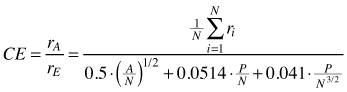 | rA – observed mean distances between trees A – area (m2) N – Total number of trees P – circumference of the plot |
| Tij (Kint 2004) | 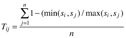 | si – size of i-th tree sj – size of j-th tree n – number of nearest neighbors (n = 3) |
| Uniform angle index Wi (Gadow and Hui 2002) |  | n – number of nearest neighbors vj = 1 if αj < α0 (α0 = 90°) otherwise: vj = 0 |
| Mean directional index Ri (Corral-Rivas et al. 2006) | 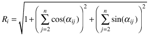 | αij – angle between i and j points |
| Index of nonrandomness Si (Pielou 1959) | λ – point density | |
| Mingling index SM (Gadow and Hui 2002) | 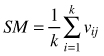 | k-numbers of nearest neighbors vij = 1 if reference tree and neighbor are different species, otherwise vij = 0 |
| Size dominance index Ui (Hui et al. 1998) |  | n – number of nearest neighbors vj = 0 if neighbor j is smaller than reference tree, otherwise vj = 1 |
| Dispersion index Iσ (Morisita 1962) | 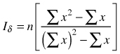 | n – sample size Σx – sum of quadrat counts (Σx)2 – sum of quadrat counts squared |
| Variance/mean ratio Ic (Krebs 1999) |  | Sn2 – variance |
| Mean of angles (Assunção 1994) |  | n – number of sampling points αi – angle between sample point and its nearest two neighbors |
| Segregation index (Pielou 1977) | m, n – numbers of species A and B | |
3.1 Quadrat counts in spatial analysis
In quadrat counts the data for analysis come from small subareas (quadrats) located in a particular region of interest. This technique is the oldest and the simplest measure of spatial patterns. Here, the exact locations of individuals are not recorded, which simplifies data collection but also limits the statistical analysis (Krebs 1999; Illian et al. 2008). The basic requirements are that the area counted is known and that the individuals are immobile during the counting period (Krebs 1999). The disadvantage of quadrat count methods is that the perceived dispersion of the point pattern may depend greatly on the scale of study and the size of the sample unit (Krebs 1999; Perry et al. 2002).
Variance-mean ratio (Ic) is one of the oldest and the simplest indices to calculate and this concept is based on the Poisson distribution. The computed variance in the number of individuals per square is related to their mean occupancy. It provides an answer to the question whether individuals in the region being analyzed are distributed randomly, regularly or in clumps. One of the properties of the Poisson distribution is that the mean and variance are equal to intensity of the point pattern (Reich and Davis 2008). Thus, for a given set of quadrat counts, if the ratio of the sample variance to the sample mean is 1, this would indicate that the counts come from a Poisson distribution. If the index Ic > 1 (the variance is greater than the mean) one can state clumping, while Ic < 1 (the variance is smaller than the mean) points out a regular distribution of individuals in the population (Krebs 1999; Fortin and Dale 2005; Reich and Davis 2008; Pretzsch 2010). To test the statistical significance of departures from the random expectation confidence envelopes using the χ2 test for n–1 degrees of freedom are calculated (Dale et al. 2002; Reich and Davis 2008). If the value of Ic is outside the critical region, the hypothesis of a random distribution of individuals should be rejected. Results of this test depend on the number of quadrats taken into analysis (Illian et al. 2008). Using this index it is not possible to make any statements about how objects are distributed in the primary units (quadrats) or what is the average spacing between the points (in case of regular pattern) or what is the average size of patch and gap (in case of clumped distribution). This index was used e.g. by Pielou (1959), Hanewinkel (2004), Paluch (2007), Szewczyk and Szwagrzyk (2010), Rosenberg and Anderson (2011).
Quadrat variance methods stem from the application of hierarchical analysis of variance to the data from grids or strips of continuous quadrats, which are blocked in a successive power of two, thus, the number of quadrats used is restricted (Greig-Smith 1952). This blocked quadrat method (later referred to as BQV) proposed by Greig-Smith (1952) and Kershaw (1977), calculates the variance of non-overlapping blocks of different sizes. To remove limitations of BQV such as limitation of block size to powers of two, dependence of results on the starting point and the lack of independence of different variance estimates, Hill (1973) developed the so-called two-term local variance methods (referred to as TTLQV). In these methods quadrats are combined in blocks of a range of sizes no longer limited to powers of two to detect the scale of patterns in a population (Ludwig and Goodall 1978). TTLQV differs from BQV in that its variance is based on overlapping blocks. Two-term local quadrat variance can be applied to data sets collected from a series of contiguous quadrats (Krebs 1999). It calculates the average of the square of the difference between block totals of adjacent pairs of block size b (Hanewinkel 2004; Fortin and Dale 2005). The variance in TTLQV is calculated as:

where x1...xn are counts of points, n is the number of quadrats, j is the number of blocks and b is block size. Krebs (1999) stated that the upper limit of block size should be n/2; however, the recommendation is n/10. Plotting variances against block size can be used to determine the spatial pattern. If individuals are distributed randomly over the population, the plot of variance against block size will fluctuate irregularly. Regularity can be stated if the variances are low and will not fluctuate with block size, while in case of the clumping pattern variances will tend to peak at the block size equal to the radius of clump size (Krebs 1999). Campbell et al. (1998) in their discussion on the interpretation of peaks in two-term form pointed out that peaks found at block sizes 1, 2 and 3 occur frequently by chance and do not indicate a pattern. Fig. 1 illustrates types of spatial patterns distinguished by TTLQV.
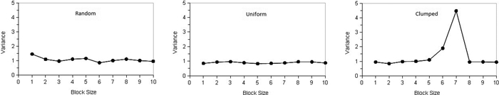
Fig. 1. Schematic illustration of the spatial pattern types for TTLQV method for contiguous quadrats: (left) random, (middle) regular and (right) clumped (adapted from Krebs 1999). View larger in new window/tab.
Another method based on quadrat variance is three-term local quadrat variance (referred to as 3TLQV), being the extension of TTLQV method. It examines the average of squared differences among trios of adjacent blocks of size b and it looks at the squared differences between the sum of the first and the third block and twice the second block. Its variance is denoted by (Dale et al. 2002; Fortin and Dale 2005):

This three-term local quadrat variance form is assumed to be less sensitive to trends in the data sets (Hanewinkel 2004). Examples of the use of TTLQV and 3TLQV can be found in Ludwig and Goodall (1978), Dale and MacIsaack (1989), Dale and Blundon (1990), Wheeler et al. (1994), Perry et al. (2002) and Hanewinkel (2004).
Morisita’s dispersion index (Iσ) is also based on counts of individuals on sample squares and it is calculated from the number of objects on the squares, number of squares and total numbers of individuals (Krebs 1999). The index is a quotient of observed probability σ for a given distribution and the expected probability E(σ) = 1/q when the distribution is random (q – number of squares). The index can take values from 0to n. If Iσ = 1 (both probabilities are equal) the population is said to be randomly dispersed; if Iσ > 1 the population shows clumping distribution and Iσ < 1 indicates regularity (Pretzsch 2010). Statistical significance of observed deviations from expectations (randomness) can be tested using critical values of the χ2 distribution with n–1 degrees of freedom (Krebs 1999). Also standardized index Iσst can be used, being the scaled Morisita’s index Iσ and setting up [–0.5, 0.5] values as 95% confidence regions around random distribution with the value 0 (Krebs 1999). The calculation of standardized Iσ is more tedious. First, the standard Iσst index must be calculated and then one needs to calculate critical values for the index describing uniformity or clustering. After calculation of these critical values the standardized Iσst index has to be calculated using four different formulas (Krebs 1999). This modified index can take values between –1 and +1. This standardized modification is assumed to be a very good measure of spatial dispersion, because it is not affected by the population density and sample size; however, it is hard to state the best sample size to provide a reliable index (Krebs 1999). This modified index was applied among others by Miyakodoro et al. (2003), Veech (2005); Taylor et al. (2006), Habashi et al. (2007), Sankey (2008) and Sapkota et al. (2009).
In literature other indices based on quadrat counts can be found, however, they are not so commonly used in practice. Hanewinkel (2004) listed such indices: the index of cluster size (ICS), index of cluster frequency, index of mean crowding, index of patchiness and Green’s index.
3.2 Nearest neighbor indices
Nearest neighbor statistics (NNS) requires information about relative tree positions in the population using an appropriate sampling method (Kint et al. 2004). Using NNS one assumes that spatial structure of forests is determined to a large extent by nearest neighbors relations. Using indices belonging to this group of methods we can determine different aspects of spatial structure: tree distribution type, species mingling and spatial differentiation of tree sizes. They are very useful in comparisons, e.g. between different forest types, managed vs. natural forests, between different harvest events, etc. (Pukkala et al. 2012).
3.2.1 Distance-dependent indices
These methods are based on nearest-neighbor distances. The measurements are of two types: distances from the sample point to a tree or from a tree to a tree (Staupendahl and Zucchini 2006). These indices can be also applied for data sets with known tree positions.
The Clark-Evans index of clumping (CE) belongs to the methods based on distances between individuals within the population. It was introduced by Clark and Evans (1954) and then modified by Donnelly (1978). It uses distances between nearest neighbours and it is measured for all individuals located on the plot. This index is a measure of the extent, to which the observed population differs from the randomly distributed one. The maximum value of the index is reached for a strict hexagonal pattern and then CE = 2.15 for (Krebs 1999; Neumann and Starlinger 2001). Its interpretation is easy: a population distributed randomly shows CE = 1.0, while regularity can be assumed if CE > 1.0. Index CE < 1.0 indicates the clumped distribution of individuals. A simple test of significance for the deviation from randomness can be estimated using the Z-test (Clark and Evans 1954; Krebs 1999; Pommerening 2002). Donnelly (1978) modified the CE index in terms of the edge effect correction. This index can be used as a preliminary step of the analysis and provides information about the point pattern in a fine spatial scale (at nearest neighbour distances). As it was stated by Longuetaud et al. (2008), this index is density-dependent and comparisons between results from populations of varying densities are rather difficult. Kint et al. (2003) pointed out that the CE index should not be applied in populations, for which clustered distribution can be assumed. In such cases other indices can be more suitable. This index is, however, quite frequently used in forestry – see Pretzsch (1997), Pommerening (2002), Kint et al. (2003), Kint et al. (2004), Vorčák et al. (2006), Szmyt and Ceitel (2011) and Szmyt (2012).
The Pielou index of nonrandomness (Si), alternatively to CE, uses the distance from random points selected in the area under investigation to their nearest neighbor. In case of random distribution, the distribution of random points is as random as trees are. The value of Si > 1 indicates clustering, while Si < 1 points out regularity in spatial distribution. Randomly spaced individuals show values of Si being around 1 (Pielou 1959). The significance of any deviations from the expected value for the Poisson distribution can be tested using χ2 distribution with 2n degrees of freedom (n – number of distance measurements). Payandeh (1974) gave an example of this index applied to forests located in Ontario, Canada.
3.2.2 Angle-based indices
The uniform angle index (Wi), also referred to as the contagion index, describes the degree of regularity in spatial distribution of individuals (Gadow and Hui 2002). Unlike CE, the contagion index is based on the classification of angles between nearest neighbours of the reference point (event) (Pommerening 2002; Aguirre et al. 2003; Corral-Rivas et al. 2010). If Wi = 0, then one can assume that objects close to the reference point (tree) are distributed in a regular manner and Wi = 1 indicates a clumped distribution. If the so-called structural group of 4 nearest neighbors (Fig. 2) are taken into account, Wi can take five values (0; 0.25, 0.5; 0.75 and 1; Fig. 3). The distribution of index values provides a more detailed analysis of the observed population, not only in terms of a single mean parameter (Pommerening 2002). The significance of deviations from CSR can be estimated by a comparison of the index value with the critical values Wiα and Wi1-α (α – the level of significance). If empirical Wi is larger than Wiα, the CSR hypothesis is rejected in favor of clustering of points. If Wi is smaller than Wi1-α, then points are distributed regularly. As Corral-Rivas et al. (2006) stated the contagion index is a very rapid and cost-effective method to characterize the spatial structure of any population, because it requires neither the distance nor angle measurements (angles are classified, not measured exactly). The authors also stated that this index is a powerful tool when 100 objects (or more) are present on the plot. This index is also plot-shape independent. Examples of application of the contagion index can be found in Pommerening (2002), Aguirre et al. (2003); Montes et al. (2004), Corral-Rivas et al. (2006), Staupendahl and Zucchini (2006), Pommerening (2006), Pastorella and Paletto (2013). The critical values Wiα and Wi1-α determined by simulations depend on the number of points on the plot, but not on its size (Corral-Rivas et al. 2006).
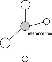
Fig. 2. An example of structural group of trees for calculation of uniform angle index (Wi), size differentiation index (T) and species mingling index (SM) (Pommerening 2002).
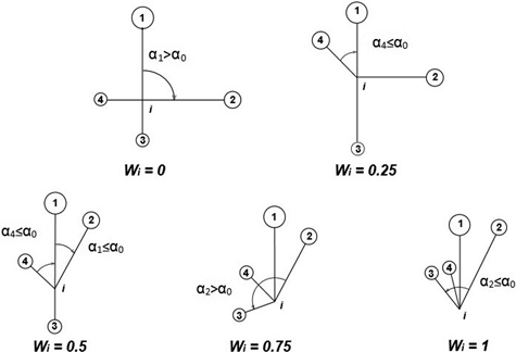
Fig. 3. Calculation of uniform angle index Wi and possible values for structural group of 4 neighbors around the reference i-tree (Gadow and Hui 2002).
The mean directional index (Ri) is similar to Gadow’s index and it does not require measurements of tree-to-tree distances. It characterizes the neighbourhood of a reference point (e.g. tree) by the directions, under which the nearest neighbors are visible (Corral-Rivas et al. 2006, Fig. 4). The behaviour of the index corresponds to Wi and if individuals are regularly spaced Ri = 0, whereas when they are distributed in clumps the index Ri tends to take larger values. The value for a random population is Ri = 1.779. It shall be deemed that this index is a powerful method in the recognition of random, regular or clumped distributions when the number of individuals in a population exceeds 50. Testing for CSR is similar as for the Wi index. Examples of the use of the Ri index can be found in Corral-Rivas et al. (2006) and Illian et al. (2008).
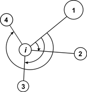
Fig. 4. Illustration of angle measurements for mean directional index Ri with structural group of 4 neighbors around the reference i-tree (Corral-Rivas et al. 2006).
The mean of angles (θ) presented by Assunção (1994) is another angle method to test the hypothesis of complete spatial randomness in point distribution. It considers individuals represented by points occurring in a planar region (study plot). A sample of n point locations is selected and two nearest points (events) to each of the sample points are found. The test for CSR is based on the angle between vectors connecting each sample point to its two neighbors. The index can take values between 0and π if the points are distributed according to CSR then mean θ = 90°. For a regular distribution θ > 90°, for a tendency towards clumping θ < 90°. Then, the power of the test is compared with the Hopkins and T2 test (Assunção 1994; Assunção and Reis 2000; Staupendahl and Zucchini 2006; Trifković and Yamamoto 2008). The authors recommended this method as especially useful in ecological studies in regions where distance measurements are difficult to conduct; however, it is not so commonly used as other indices described above.
3.2.3 Spatial indices for tree attributes
Simple spatially explicit indices can be also used to describe the distribution of individuals of different types described by marks assigned to them. Such information reveals the impact of interactions (e.g. competition) between objects. Below several such indices are described.
Spatial differentiation of sizes (T) is often calculated for quantitative attributes of individuals (sizes, e.g. diameters, heights, crown width) and it reflects size differentiation between neighboring objects. Index values can vary between 0(no differentiation) and 1 (complete differentiation) (Pommerening 2002). Again, a single value of the index provides information on the average differentiation of individual sizes in a certain population. More informative is the distribution of the index in differentiation classes. For 4 nearest neighbors the following differentiation classes can be applied (Aguirre et al. 2003; Kint 2004; Vorčak at al. 2008): 0.00–0.20 – very small differentiation, 0.20–0.40 – small differentiation, 0.40–0.60 – obvious differentiation, 0.60–0.80 – large differentiation and 0.80–1.00 – very large differentiation. There is no theoretical test to investigate the significance of differences between observed differentiation and under the random condition, however, the permutation procedure can be used to state such differences (Kint 2003). Examples for the application of size differentiation index are included in Kint et al. (2003); Vorčák et al. (2006); Mason et al. (2007); Sterba (2008); Barbeito et al. (2009), Crecente-Compo et al. (2009); Pommerening et al. (2011), Szmyt (2012) and Pastorella and Paletto (2013).
Size dominance indices (Ui) were proposed by Hui et al. (1998) to relate the relative dominance of a certain individual to its immediate neighbors. It is defined as the proportion of the n nearest neighbors of a given reference object which are smaller than the reference one. Similar to the differentiation index, the dominance index can take n + 1 values (n – the number of neighbors): 0(all neighbors are smaller than the reference tree), 0.25, 0.5, 0.75 and 1 (none of the neighbors are smaller than the reference tree). These classes correspond to social classes of tree position in the stand developed by Kraft. Examples can be found in Aguirre et al. (2003), Pommerening (2006) and Pommerening and Stoyan (2008).
There are also indices making it possible to describe the relative position of different qualitative marks of points (trees), e.g. tree species in mixed forests. Pielou’s index of segregation and the mingling index are the most commonly applied indices in such cases.
Pielou’s index of segregation (S), developed by Pielou (1961), describes the relative mixing of two species regardless of their spatial pattern. This method is based on the nearest neighbor distances and compares the observed number of mixed pairs with the one expected under random conditions (Kint et al. 2003, Table 2). Values of the S index vary between –1 and 1. If 0< S < 1 indicates that the nearest neighbors are always different species (spatial separation of species) and if –1 < S < 0, spatial association between two species is observed. If both species are randomly distributed, then S = 0. It is worth noting that the terms “separation” and “attraction” describe only the spatial patterns of both species. To judge whether the observed mixture departs significantly from the case of random conditions the χ2 test may be used. The spatial segregation index was applied by Kint et al. (2003), Kint (2005), Getzin et al. (2006), Bilek et al. (2011), Pastorella and Paletto (2013).
| Table 2. Contingency table summarizing the number of trees of both species (A and B) with the nearest neighbors of their own species (a and d) and of the other species, used for Pielou’s segregation index calculation (Pielou 1977). | ||||
| Species of the nearest neighbor | ||||
| A | B | Total | ||
| Reference species | A | a | b | m |
| B | c | d | n | |
| Total | v | w | N | |
| Explanation: m = a + b; n = c + d; v = a + c; w = b + d; N = m + n | ||||
Spatial mingling index (SM) differs from the S index in such a way that in this case multiple neighbors can be accounted for and the index is not limited to the mixture of only two species, but it can be estimated for all species together as well as for each species separately (Gadow and Hui 2002). The index gives the proportion of neighbors of the reference tree which are not the same species. Hence, in case of 4 neighbors the index can take five values: 0, 0.25, 0.5, 0.75 and 1, depending on the spatial pattern and relative frequency of the species. Strongly represented or segregated species result in low SM values and less frequent or regularly spaced species have higher values of the SM index (Aguirre et al. 2003; Kint at al. 2003). Low values of the index indicate homogenous groups of species and low mingling, while high values indicate complete mixture of the species. To find out if the observed spatial mingling is different than in case of a random situation Kint (2004) suggested the application of the permutation procedure. The distribution of the mingling index provides more detailed insight into the spatial composition of the forest. Pommerening (2002); Graz (2004); Bilek et al. (2011); Ruprech (2010), Pommerening et al. (2011) and Pastorella and Paletto (2013) applied this index in different forest studies.
4 Functional statistics in spatial analysis
The modern point process statistics uses functions instead of simple indices described above. These functions depend on distances between all individuals in the population (e.g. K-function, L-function, and pair correlation function) or nearest-neighbor distances (e.g. G-function, F-function and J-function). Thus they can be used to detect simultaneously different spatial scales of the observed pattern (Ripley 1981; Illian et al. 2008). This is a great advantage over the nearest neighbor indices. Their disadvantage is that they usually require much more detailed field data sets, namely maps of locations of individual specimens. On the one hand it makes the analysis more precise, but on the other hand, gathering data is much more costly and time consuming. Recorded results are then related to theoretical (reference) distributions (null models). Usually a homogenous Poisson model (assuming randomness of point distribution) is such reference in the first stage of each analysis. Thanks to revealing the spatial pattern at different spatial scales simultaneously, it is possible to distinguish different processes responsible for creating a certain spatial structure of the population.
The nearest-neighbour distance distribution function (G-function) is based on distances from an event (e.g. tree) to its nearest neighbor and it measures the distribution of these distances. The function can be estimated as:
![]()
where the nominator is the number of points si with the nearest neighbor distance rmin ≤ r and the denominator is the number of points in the study area. Under the CSR the G-function is (Mateu et al.1998; Bivand et al. 2008; Illian et al. 2008):
![]()
where λ is intensity (the mean number of events per unit area).
The empirical G-function is then plotted against the theoretical expectation. The shape of the function indicates how the events (trees) are spaced in a point pattern. If they are clustered, then the G-function increases rapidly at the short distances, while it increases slowly up to the distance where most of events are spaced and then it increases rapidly (regularity). The significance of departures from the CSR hypothesis can be evaluated using simulated confidence envelopes computed by a repeated simulation of the CSR point process with the same intensity λ from the study region and check if the empirical function is inside the envelopes (Dixon 2001; Bivand et al. 2008). The application of the G-function is not so common, but it may be seen in Mateu et al. (1998), Dixon (2001) and Wiegand et al. (2012). Fig. 5 presents an example of the G-function calculated for 43 year old pines regenerated by planting at a certain initial spacing. It indicates regularity of up to 0.5 m reflecting the initial spacing between plants.
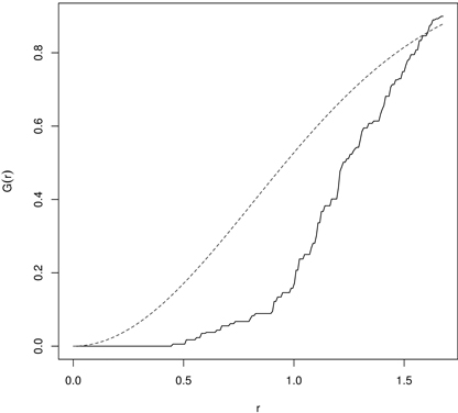
Fig. 5. The G-function calculated for 43 year old Scots pine semi-plantation indicating regularity (dashed line – the G-function for randomness (CSR); solid line – empirical G-function).
The empty space function (F-function) (also called spherical contact distribution) is based on measures of distribution of all distances between arbitrary selected points (but not the location of trees) on the plane to their nearest neighbor and it is closely related to the G-function (Mateu et al. 1998; Dixon 2001; Bivand et al. 2008; Illian at al. 2008). The name “empty space function” results from the fact that it is a measure of the average space between points. Under the CSR assumption the function is:
![]()
Then the empirical F-function is compared with a theoretical one by simulation of the envelopes (Monte Carlo procedure). Points are clustered if F(r) rises slowly at a small distance and then rapidly at longer distances. Regularity is assumed when F first rises rapidly and then slowly at longer distances. So interpretation of the F-function is thus reverse to the G-function. For examples of applications of the empty space function see references to the G-function. Wiegand et al. (2012) stated that both functions can also quantify aspects of non-stationary patterns, when the pattern comprises areas with low and high densities of points. Fig. 6 presents the F-function calculated for yews (Taxus baccata L.) indicating their clumping distribution.
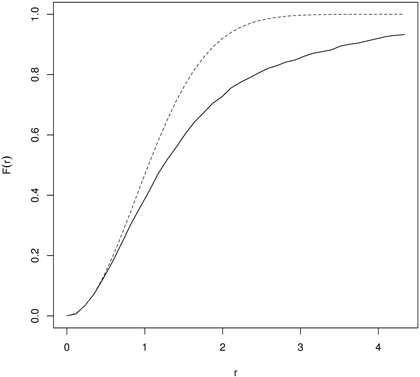
Fig. 6. The F-function for naturally regenerated English yew (Taxus baccata L.) trees indicating clustering (dashed line – the F-function for CSR; solid line – empirical F-function).
Both functions, G and F, require the edge correction procedure. Different methods to solve this problem can be found in textbooks of Ripley (1981) and Illian et al. (2008).
The J-function is another distance-dependent function for analysis of the spatial point pattern (Van Lieshout and Baddeley 2006). The idea of this function is to compare distances from an arbitrary point to the nearest neighbor (empty space F-function) and distances from typical point of the pattern measured by the nearest-neighbor distance G-function. This can be written as:

where F(r) is the empty space function; G(r) is the nearest-neighbor distance function.
Then, if J(r) ≡ 1 the distance distribution follows the Poisson process. Deviation J(r) > 1or J(r) < 1 indicates spatial regularity and clustering, respectively (Van Lieshout and Baddeley 1999; Paolo et al. 2002; Fortin and Dale 2005; Van Lieshout and Baddeley 2006). Because practically observation of points is restricted to some bounded area (measurement plot) the estimate of the J-function is hampered also by the edge effect. As a consequence, edge correction should be applied (Baddeley et al. 2000). The inference about the significance of departures from 1 can be done by the Monte Carlo procedure and the null hypothesis of spatial independence or random labeling can be tested. Fig. 7 is an example of the J-function indicating regularity in distribution of 60 years old beech (Fagus sylvatica L.) trees in a managed beech stand. More examples of the J-function application may be found in references cited above and also in Paolo et al. (2002) and Wu and Li (2009).
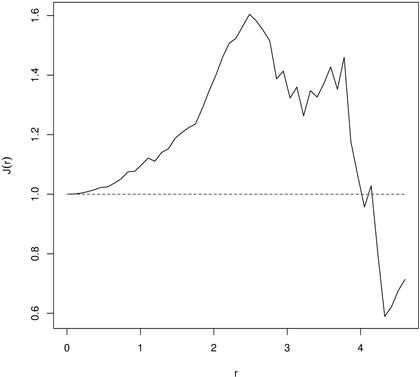
Fig. 7. The J-function indicating regular point pattern for 60 years old managed European beech stand indicating regularity (dashed line – the J-function for CSR; solid line – empirical J-function).
The G, F and J functions can be extended to analyze multivariate spatial point patterns (Van Lieshout and Baddeley 1999; Baddeley and Turner 2008; Wu and Li 2009).
The Ripley’s K function is a very common method used to examine spatial point patterns and it uses distances between all individuals in the population, not only between the nearest neighbors. It makes possible to examine and summarize a point pattern, test hypotheses on the models, estimate parameters and fit models (univariate cases) and describe relationships between two or more types of points (bi- or multivariate cases) at different spatial scales. The formula for the K-function is (Dixon 2001; Illian et al. 2008; Grey and He 2009):
![]()
and the unbiased estimator of K-function is:
![]()
where n is the total number of objects (e.g. trees) in the plot area A, uij denotes the distance between the i-th tree and j-th tree. I(uij) is an indicator function equaling 1 if uij ≤ d (or 0otherwise) and wij is edge correction factor. This function determines the consistency of the observed distribution of distances among all objects located in the spatial window (sample plot) with the theoretical distribution for the Poisson model (CSR) as a benchmark. Usually measurements are taken only on the sample plot, therefore different methods of edge effect correction should be applied to get an unbiased estimator of the function (e.g. Szwagrzyk 1992; Haase 1995; Illian et al. 2008). Results are usually presented as a graph of the K-function plotted against different distances r (spatial scales) and the shape of the graph provides valuable information on the point distribution. Because of the cumulative character of the K-function it usually indicates spurious clustering, resulting from many inter-point distances at large distances. Interpretation of the K-function is easier if one uses its standardized L(r) version, which stabilizes its variance and it is approximately constant under CSR. Its formula is (Dixon 2001):

In random populations, in literature referred to as CSR, K(r) = πr2 (L(r) = 0). If objects within the spatial window are clumped, then the K-function receives higher values (K(r) > πr2 or L(r) > 0), and if they are regularly (evenly) spaced – the K-function shows low values (K(r) < πr2 or L(r) < 0) (Illian et al. 2008; LeMay et al. 2009). In the first case the typical point is a part of the cluster and has few nearest neighbors and the local density is larger than λ. In the second variant the point is isolated from the nearest neighbors and local density is smaller than λ (Illian et al. 2008). Clustering in yew distribution based on K- and L-function is presented in Fig. 8 and Fig. 9.
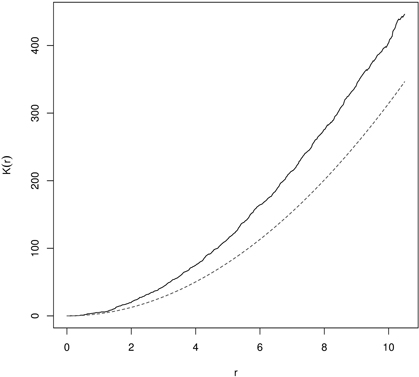
Fig. 8. Ripley’s K-function for English yew (males) trees indicating clumping distibution (dashed line – K-function for CSR; solid line – empirical K-function).
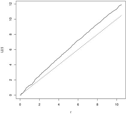
Fig. 9. The L-function for English yews (males) indicating clustering (dashed line – the L-function for CSR; solid line – empirical L-function).
Statistical tests to verify whether deviations from CSR are significant can be performed using two methods. One method relies on the constant confidence envelopes around CSR (Szwagrzyk and Ptak 1991; Haase 1995) and the second is based on the Monte Carlo procedure (Haase 1995; Wiegand and Moloney 2004; Illian et al. 2008). If the empirical function exceeds the upper (lower) simulated envelopes, the objects indicate a significant clustered (regular) distribution at a certain distance r. Usually, the rejection of the null hypothesis about CSR is enough to make the statements about the distribution of individuals in the population, but it can also lead to the application of other theoretical null models, such as the Neyman-Scott cluster model, the Strauss model, the double cluster model, etc. (Stoyan and Penttinen 2000; Wiegand and Moloney 2004; Wiegand et al. 2007).
The pair correlation function – referred to as g(r) – is a more informative second-order summary characteristic. It is related to the K-function, but it is non-cumulative in character. The relation to the K-function is (Stoyan and Stoyan 1996):

and the probability that each disc dx and dy contains an object of the process is:
![]()
For a random population g(r)≡1, the clustered population g(r) > 1 and the regularly spaced population g(r) < 1. The pair correlation function can take any value from 0to infinity. For large distances g(r) trends to be 1. This function identifies the distances, at which (not to which, as in the cumulative K-function) deviations from CRS occurs (Pretzsch 2010). The pair correlation function is a suitable tool to indicate a range of correlation, the distance up to which individuals interact with one another. In the cluster process the correlation range describes the size of clusters (cluster diameter). In case of a regular process (inhibition process) g(r) indicates the minimum distance (g(r) = 0) between objects (the so-called hard-core distance) (Illian et al. 2008). Similarly to the K-function, envelope tests based on the Monte Carlo procedure can be used to detect the significance of departures from 1 (Stoyan and Stoyan 1996; Illian et al. 2008; Getzin et al. 2011). Fig. 10 presents the typical shapes of g(r) for different types of distribution.
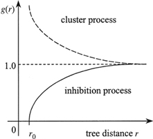
Fig. 10. Shape of pair correlation g-function for different types of point patterns (dashed line – the g-function for CSR; dashed line – clustering; solid line – regularity) (Pommerening 2002).
Both functions can be extended to bi- or multivariate forms, facilitating interpretation of interactions between different types of individuals (e.g. tree species, different sizes, sexes, etc.). These forms are shortly described below.
The bivariate K-function is defined as the expected number (E) of n-type points within the distance r of an arbitrary point of type m divided by the intensity of n-type points (Wiegand and Moloney 2004):
![]()
where E is the expectation operator.
The estimator of bivariate K-function is:

It indicates attraction between two types of objects if more than the expected number of 2-type points occur close to 1-type points (K12(r) > πr2). If the reverse is true (K12(r) < r2), then repulsion between two different types of individuals can be stated. In case of K12(r) = πr2 both types of objects are spatially independent (Wiegand and Moloney 2004; Getzin et al. 2006; LeMay et al. 2009). Again, interpretation is easier when the L12(r) modification is used. Then:

values L12(r) > 0points out the attraction between different types and L12(r) < 0indicates repulsion (separation) between them. L12(r) = 0states spatial independence between objects of different types (Wiegan and Moloney 2004).
The bivariate pair correlation function – gnm(r) – is an analogue of Ripley’s bivariate one (Wiegand and Moloney 2004):

A general interpretation of the bivariate pair correlation function is as follows: for gnm(r) = 1 spatial independence of two types of points is stated, if gnm(r) > 1 – attraction and gnm(r) < 1 – repulsion between individuals of different types is observed. Significance of the deviations from the null model is estimated by the Monte Carlo procedure.
5 Testing complete spatial randomness – envelope or deviation tests?
Testing the hypothesis of CSR is important for exploratory analysis in point process statistics. Acceptance of CSR means that a given point pattern has two main features: there is no need to use models more complicated than the Poisson one, and it is not possible to find causes of an interaction between points based on geometry of the observed pattern alone (Illian et al. 2008, p. 83). It is known that in natural populations a true Poisson pattern is seldom observed, so the CSR hypothesis means that the analyzed pattern is only close to the Poisson process model. If the CSR is rejected, then other models have to be searched for.
Tests are based on the differences between values of the test function obtained from the field data and theoretical values. A problem occurs when one wants to handle these differences for different distances. In point process statistics simulation envelope test and deviation test can be used in testing the null hypotheses and both of them are Monte Carlo significance tests (Grabarnik et al. 2011; Myllymäki et al. 2013a). Avoiding statistical details these tests are shortly described below.
The envelope test is based on some functional summary characteristics, e.g. the K-function or L-function. The idea of this test is to compare observed summary characteristic obtained from the observed pattern to estimates from simulations upon the null model, using the estimated parameters in the same window. The null model is usually simulated n times and the estimate of Kmin(r) and Kmax(r) of estimator ![]() , for i = 1…k, is calculated for each simulation. Extreme values from the simulations are determined and plotted together with
, for i = 1…k, is calculated for each simulation. Extreme values from the simulations are determined and plotted together with ![]() . Kmin(r) and Kmax(r) are usually called envelopes of estimator
. Kmin(r) and Kmax(r) are usually called envelopes of estimator ![]() (Illian et al. 2008; Grabarnik et al. 2011). Then, if
(Illian et al. 2008; Grabarnik et al. 2011). Then, if ![]() exceeds upper or lower envelopes at distance r, the null hypothesis is rejected for that distance r, otherwise the null model holds. Grabarnik et al. (2011) stated that the choice of a suitable number of simulations for constructing envelopes is difficult, because the I-type error (rejection of the null hypothesis even though it is true) is not known a priori. A single distance test (for a certain distance) and the global test for all distances can be very different. Many tests, one for each distance, result in weaker than expected statistical performance (Loosmore and Ford 2006; Illian et al. 2008). Usually envelope tests require a large number of simulations (e.g. n = 999) to be the minimum for obtaining the I type error probability close to 5% (Grabarnik et al. 2011). Myllymäki et al. (2013a) propose new global envelope tests providing both the p-value and the graphical representation. This new method offers a new way to calculate the global envelope test on the whole range of distances and is based on the ordering of the test function (e.g. the K-function) and the simultaneous envelopes, which have the graphical interpretation. It facilitates the rejection of the null hypothesis even if the data function is not completely inside the constructed envelopes. If the data function is outside the rank envelopes (based on ranking the test function) for some distance, the null model is to be rejected. Simultaneously the envelopes show the distances where the data function denies the null hypothesis. More details on this new approach can be found in Myllymäki et al. (2013a).
exceeds upper or lower envelopes at distance r, the null hypothesis is rejected for that distance r, otherwise the null model holds. Grabarnik et al. (2011) stated that the choice of a suitable number of simulations for constructing envelopes is difficult, because the I-type error (rejection of the null hypothesis even though it is true) is not known a priori. A single distance test (for a certain distance) and the global test for all distances can be very different. Many tests, one for each distance, result in weaker than expected statistical performance (Loosmore and Ford 2006; Illian et al. 2008). Usually envelope tests require a large number of simulations (e.g. n = 999) to be the minimum for obtaining the I type error probability close to 5% (Grabarnik et al. 2011). Myllymäki et al. (2013a) propose new global envelope tests providing both the p-value and the graphical representation. This new method offers a new way to calculate the global envelope test on the whole range of distances and is based on the ordering of the test function (e.g. the K-function) and the simultaneous envelopes, which have the graphical interpretation. It facilitates the rejection of the null hypothesis even if the data function is not completely inside the constructed envelopes. If the data function is outside the rank envelopes (based on ranking the test function) for some distance, the null model is to be rejected. Simultaneously the envelopes show the distances where the data function denies the null hypothesis. More details on this new approach can be found in Myllymäki et al. (2013a).
The deviation test transforms information from the functional summary statistic (e.g. the K-function) into the scalar test statistic by calculating a measure of deviation between the observed (or simulated) function and the expectation under the null hypothesis (Grabarnik et al. 2011). The deviation tests resolve multiple hypothesis testing by summarizing differences between the observed and theoretical functions for all analyzed distances into a single number by the so-called deviation measures (Myllymäki et al. 2013b). Two types of deviation measure (u) being applied are the integral and maximum one, which correspond to two-sided envelope tests (Grabarnik et al. 2011). After calculation of the deviation measure for the observed and simulated data, the p-value of the deviation test can be easily estimated (Loosmore and Ford 2006; Grabarnik et al. 2011). This estimate is based on the rank of the deviation measure among all the values of u and its precision can be calculated, since each possible ranking of u is equally likely under the null model (Grabarnik et al. 2011). Although the deviation test overcomes the multiple testing problem (occurring in envelope tests) due to the simultaneous verification of the test function for all distances analyzed, it is sensitive to unequal variance and asymmetry of the test function over all analyzed distances (Myllymäki et al. 2013b). A disadvantage of this test is that it does not indicate the distance, at which the rejection of the null hypothesis is possible and it is rather impossible to detect the reasons why the data set contradicts the null model (Grabarnik et al. 2011; Myllymäki et al. 2013b). The application of the deviation test must involve three steps: choosing a suitable test function (e.g. K-function, the F-function, etc.), choosing the suitable transformation of the summary function or scaling of the differences, and calculation of the global deviation measure (Myllymäki et al. 2013b). Fig. 11 shows the pair correlation function and the critical region based on 199 Monte Carlo simulations for clustered distribution of yew seedlings.
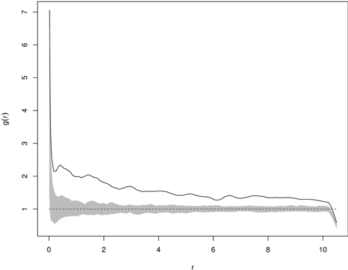
Fig. 11. Example of g(r) function for statistically significant clumped distribution of yew seedlings (solid line – empirical g-function; shaded area – critical region based on 199 Monte Carlo simulations; dashed line – g-function for CSR).
6 Suitable null models prevent misinterpretations
A successful application of Ripley’s or pair correlation functions is to select a suitable null model, with which the empirical function is compared (Degenhardt 1999; Wiegand and Moloney 2004; Illian et al. 2008; Bieng et al. 2011). In other words, the statistical test makes it possible to find out if the observed point pattern has characteristics similar to those of a specified null model. In ecological analysis the simplest and the most commonly used null model is the homogenous and isotropic Poisson model corresponding to the CSR hypothesis. This model assumes that each point of the process has the same intensity of occurring at any place in the studied region and the position of a point is independent of the position of other points (no interactions between points exist). If the first stage of the analysis indicates that the CSR hypothesis should be rejected, then other classes of models have to be implemented (e.g. Cox models, Gibbs models, etc.). The choice of the suitable model is not easy. Illian et al. (2008) indicated that information on clustering or regularity observed at different spatial scales combined with a priori knowledge may indicate which class of models are the most appropriate. They underlined that – as a general rule – in the first step one should use the basic classical models, since they can be easily fitted and simulated. Once the model is fitted to the data, goodness-of-fit tests should be performed to assess the model suitability (Loosmore and Ford 2006; Wiegand et al. 2007; Illian et al. 2008; Grabarnik et al. 2011). It is worth noting that functions described above have two main assumptions: homogeneity and isotropy of the process. The first assumption refers to a lack of significant differences in intensity (first-order property of the process) of the population and the second means that the process is invariant with respect to rotations. To deal with non-homogenous populations, other null models (e.g. a heterogeneous Poisson model) or delineating homogenous sub-regions into homogenous regions are required (Wiegand and Moloney 2004).
Applications of other than CSR null models can be found in Boyden et al. (2005), Camarero et al. (2005), Wiegand et al. (2007), Jacquemyn et al. (2009), Comas et al. (2009), Law et al. (2009), Picard et al. (2009), Wiegand et al. (2009), Eichhorn (2010), Martínez et al. (2010), Zhang et al. (2010) and Réjou-Méchain et al. (2011).
7 Marks and mark hypothesis testing
The raw analysis of spatial patterns of individuals is often supported by the analysis of spatial patterning of their attributes (Mateu 2000; Illian et al. 2008). Assigning marks to the points facilitates the use of methods from the field of marked point process statistics. Different correlation functions described below can be applied for that.
The mark connection function (pij) is applied to analyse correlations between qualitative (e.g. species, sexes, etc.) marks (Gavrikov and Stoyan 1995; Illian et al. 2008). It is a measure of the dependence between the types of two points (e.g. two species) of the process. The value of pij is interpreted as “the conditional probability that two points at distance r have marks i and j, given that these points are in the point process N” (Illian et al. 2008). If marks attached to points are independent and identically dispersed, then:
![]()
where pi denotes the probability that the point is of type i. If pij > pi(r)pj(r), then a positive association between two types of points can be stated, while smaller values of pij indicate a negative association (Gavrikov and Stoyan 1995). Examples of the use of the mark connection function can be found in Gavrikov and Stoyan (1995), Paluch and Bartkowicz (2004), Illian et al. (2008), Raventós et al. (2010) and Pommerening et al. (2011). It should be noted that bivariate pair correlation functions gij(r) and pij(r) provide different information, although they describe relations between two types of points. Due to the small number of pairs of points of both types as well as the small number of points in general at a certain inter-point distance gij(r) can take small values, while pij(r) can still be close to 1 if the pairs of points are mainly of both types i and j (Illian et al. 2008, p. 332).
Individuals can be described not only by qualitative marks, but also quantitative marks (e.g. diameter, height, crown width, etc.) can be attributed to points (Penttinen et al. 1992; Gavrikow and Stoyan 1995; Stoyan and Penttinen 2000; Penttinen 2006; Illian et al. 2008). Correlations between these types of marks can be analyzed by the mark correlation function and the mark variogram and both functions can answer different ecological questions.
The mark correlation function – kmm(r) – relies on inter-point distances in a population and it considers correlations among marks relative to the case of independent marks. It helps to detect correlations in the sense of mutual stimulation or inhibition of individuals (Pommerening 2002; Illian et al. 2008). The mark correlation function is a conditional association of marks and the expectation is conditional (Eox) on that there is a point at o and x at the inter-point distance r (Penttinen et al. 1992; Pommerening 2002; Penttinen 2006).
![]()
This function is scaled by dividing by squared mean mark (µ) to make the interpretation easier (Gavrikov and Stoyan 1995; Illian et al. 2008; Grabarnik et al. 2011):
If marks assigned to points are independent, then the function is equal to 1 for all distances. If kmm(r) > 1 it means that points located apart at distance r tend to have on average a larger mean mark indicating a mutual stimulation or positive correlation. An opposite situation, kmm(r) < 1, indicates mutual inhibition between points (negative correlation) and points tend to have on average smaller marks than the mean mark for the population (Illian et al. 2008; Getzin et al. 2008; Wälder and Wälder 2008; Grabarnik et al. 2011; Ledo et al. 2011). In plant populations inhibition results mostly from competition between close individuals, resulting in smaller values of their marks (e.g. diameter, height). Mutual stimulation suggests that individuals benefit from being close to each other. This type of a correlation function is a good tool to verify the strength of competition in such cases when competition does not result in the death of individuals, but it only reduces their growth.
The mark variogram – γ(r) – makes it possible to answer the question whether individuals are similar or different at a certain distance r from one another. This function is suitable to identify the effect of interactions between points (e.g. plants, trees) and environmental factors on their sizes. It characterizes squared differences between marks (m) of pairs of points within the distance of r under the condition that there are points at locations x and x + r (Stoyan and Penttinen 2000; Stoyan and Wälder 2000; Suzuki et al. 2008; Gonçalves et al. 2011; Pommerening and Särkkä 2013):
![]()
It has small values if the marks are similar (positive autocorrelation, similar sizes of nearest neighbours) at a certain distance r, and large values if they differ strongly (negative autocorrelation, large and small individuals are close to each other). The mark variogram provides two important characteristics: the range of correlation and the strength of interaction. The definition of a mark variogram is very similar to that in geostatistics. The difference is that a mark variogram is measured at some specific locations (trees) not for the whole space, and that is why the shape of a mark variogram can be different from that of a geostatistical variogram (Illian et al. 2008; Pommerening and Särkkä 2013). Fig. 12 presents kmm(r) and γ(r) for the same old-growth mixed forest in Poland. Mutual stimulation indicated by kmm(r) at small distances corresponds to small values of γ(r), indicating that the nearest neighbors are similar in size.
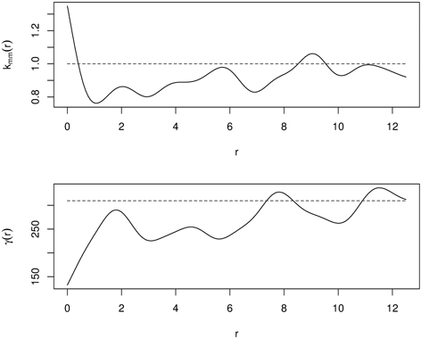
Fig. 12. Mark correlation function (kmm(r)) and mark variogram (γ(d)) for old-growth mixed forest (dashed line – independence in mark correlation; solid line – empirical functions).
In univariate analysis (regardless of the marks of points) the null hypothesis is pretty simple. The question is then whether the observed data set follows properties assigned to the selected null model. In bivariate spatial analysis (the marked point process) this is not the case, because ecologists are interested in spatial relationships between individuals in the population. The answer to the question focused on biological processes at the origin of a certain spatial pattern in the population seems to be crucial (Goreaud and Pélissier 2003; Wiegand and Moloney 2004). Goreaud and Pélissier (2003), Rozas et al. (2009), Illian et al. (2008), Grabarnik et al. (2011) stated that at least two different null hypotheses can be considered: independence (also called random superposition) and random labeling. Wiegand and Moloney (2004) propose also the third null hypotheses – antecedent conditions.
Spatial independence assumes a priori that there are two different and independent point patterns in the same spatial window assigned to two different types of points. The typical example for this hypothesis is the distribution of two species in a forest, different age categories, etc. In the spatial context it means that the position of points of type 1 (one population) must be independent of the position of type 2 (another population). Thus, the absence of an interaction between two types of points corresponds to the absence of interaction between two type patterns (Wiegand and Moloney 2004). The random labeling hypothesis means that points in an originally non-marked point process are marked independently (a posteriori marking). Concerning the spatial structure it states that the probability that one event occurs is the same for all points taken together (non-marked point process) and it does not depend on the neighbors. Here, a lack of interaction between two types of points corresponds to a lack of interaction in the occurrence of marks. A good example of the use of a random labeling hypothesis is the distribution of dead and living trees (the so-called random mortality hypothesis), infected vs. non-infected trees, healthy vs. ill trees, etc. (Goreaud and Pélissier 2003; Illian et al. 2008). Antecedent conditions can be applied for situations when two types of points are not created at the same time, but in sequence. It means that the spatial pattern of the 2nd type of points does not influence the pattern of the 1st type of points, but the type 1 pattern influences the 2nd type pattern. Thus this null hypothesis involves the time aspect (Wiegand and Moloney 2004). Multitype spatial point patterns with hierarchical interactions were also considered by Högmander and Särkkä (1999).
Examples of applications of different functions mentioned above can be found in Kuuluvainen et al. (1996), Kenkel (1997), Rozas (2003), Getzin et al. (2006), Wiegand et al. (2007), Illian et al. (2008), Suzuki et al. (2008), Wälder and Wälder (2008), Gray and He (2009), Nuske et al. (2009), Picard et al. (2009), Rozas et al. (2009), Zhang et al. (2010), Ledo et al. (2011); Nanami et al. (2011), Iszkuło et al. (2012) and Pommerening et al. (2013).
8 Recommended software for spatial analysis
Up to now there have been few software packages which can be applied in spatial analysis of populations. They differ from each other in terms of data set collection, types of data needed, methods of spatial analysis, time consumption and easiness of interpretation of results. The list below is subjective and expresses the opinion of the author of this paper.
- “Spatstat” package (Baddelley and Turner 2005) – the most commonly used statistical package for spatial analysis running in the R environment (R Development Core Team 2008). It provides creation, manipulation and plotting of point processes, exploratory data analysis, model fitting, hypothesis testing, etc. Other less known, but useful R packages such as “Spatial”, “Ecespa” or “ADS” also need to be mentioned here.
- “Crancod” (Pommerening 2012) – calculates simple structural indices as well as correlation functions. Suitable for rectangular and circular plots. Together with spatial analysis, non-spatial statistics are simultaneously calculated. Output files can be converted into easy to read spread sheets for further calculations and manipulations depending on the user’s needs.
- “spPack” (Perry 2004) – facilitates point pattern analysis in Excel with the Visual Basic for Application language. Both first-order and second-order tests are available. Also other tests, not mentioned in this paper, such as Moran’s I index and variograms are available.
- “SPPA” (Haase 1995) – simple and easy to use software to calculate Ripley’s functions (uni- and bivariate ones). It makes it possible to calculate isotropic as well as anisotropic functions. Analysis can be conducted only for data sets from rectangular plots. Makes it possible to compute goodness-of-fit tests.
- “Programita” (Wiegand and Moloney 2004) – more and more commonly used in ecological analysis. It performs univariate and bivariate point pattern analysis with Ripley’s and O-ring statistics, makes it possible to use standard and non-standard null models (the heterogeneous Poisson model, cluster models, hard and soft core models) for univariate and bivariate analysis. It is also possible to test different null hypotheses (CSR, different versions of random labeling, spatial independence, antecedent conditions). The latest version enables to compute the mark correlation function.
- “Passage – Pattern Analysis, Spatial Statistics and Geographic Exegesis” (Rosenberg and Anderson 2011) – this software is designated to make complex spatial pattern analysis, first- and second-order tests, correlogram analysis, spatial autocorrelation, variograms, etc.
- “SIAFOR” – Structural Index Assessment in Forest stands (Kint 2004) – software designed for the calculation of nearest neighbor structural indices (the Clark-Evans index, contagion index, size differentiation indices, mingling indices) in sample plots of different shapes (circular, rectangular, convex tetragonal plots) with completely stem-mapped data sets. This software can be also used as a sampling simulator.
Acknowledgements
I would like to thank Andrzej M. Jagodziński (Institute of Dendrology, Polish Academy of Sciences, Kórnik) for the motivation to write this article; Anna Binczarowska for revising the English writing. I wish also to thank the two anonymous reviewers for valuable suggestions and comments on earlier version of the manuscript.
References
Aguirre Ol., Hui G.Y., Gadow K. von, Jimenez J. (2003). An analysis of spatial structure using neighbourhood-based variables. Forest Ecology and Management 183: 137–145. http://dx.doi.org/10.1016/S0378-1127(03)00102-6.
Assunção R. (1994). Testing spatial randomness by means of angles. Biometrics 50: 531–537. http://dx.doi.org/10.2307/2533397.
Assunção R., Reis I.A. (2000). Testing spatial randomness; a comparison between T2 methods and modifications of the angle test. Brazilian Journal of Probability and Statistics 14: 71–86.
Baddelley A., Turner R. (2008). Analysing spatial point patterns in R. Workshop notes version 3. CISRO and University of Western Australia.
Baddeley A., Kerscher M., Schladitz K., Scott B.T. (2000). Estimating the J function without edge correction. Statistica Neerlandica 54: 315–328. http://dx.doi.org/10.1111/1467-9574.00143.
Bagchi R., Henrys P., Brown P.E., Burslem D.F.R.P., Diggle P.J., Gunattileke S.C.V., Gunattileke N.I.A.U., Kassim A.R., Law R., Noor S., Valencia R.L. (2011). Spatial patterns reveal negative density dependence and habitat associations in tropical trees. Ecology 92(9) 1723–1729. http://dx.doi.org/10.1890/11-0335.1.
Barbeito I., Ca-ellas I., Montes M. (2009). Evaluating the behavior of vertical structure indices in Scots pine forests. Annals of Forest Science 66: 709–719. http://dx.doi.org/10.1051/forest/2009056.
Bailey T.C., Gatrell A.C. (1995). Interactive spatial data analysis. Longman Scientific & Technical. 413 p.
Bieng M.A., Ginisty Ch., Goreaud F. (2011). Point process models for mixed sessile forest stands. Annals of Forest Science 68: 267–274. http://dx.doi.org/10.1007/s13595-011-0033-y.
Bilek L., Remes J., Zahradnik D. (2011). Managed vs. unmanaged. Structure of beech forest stands (Fagus sylvatica L.) after 50 years of development, Central Bohemia. Forest Systems 20(1): 122–138. http://dx.doi.org/10.5424/fs/2011201-10243.
Bivand R.S., Pebesma E.J., Gómez-Rubio V. (2008). Applied spatial data analysis with R. Springer. 374 p.
Boyden S., Binkley D., Shepperd W. (2005). Spatial and temporal patterns in structure, regenerations, and mortality of an old-growth ponderosa pine forest in the Colorado Front Range. Forest Ecology and Management 219: 43–55. http://dx.doi.org/10.1016/j.foreco.2005.08.041.
Brown C., Law R., Illian J.B., Burslem D.F.R.P. (2011). Linking ecological processes with spatial and non-spatial patterns in plant communities. Journal of Ecology 99: 1402–1414. http://dx.doi.org/10.1111/j.1365-2745.2011.01877.x.
Camarero J.J., Gutiérrez E., Fortin M.J., Ribbens E. (2005). Spatial patterns of tree recruitment in a relict pulation of Pinus uncinata: forest expansion through stratified diffusion. Journal of Biogeography 32: 1979–1992. http://dx.doi.org/10.1111/j.1365-2699.2005.01333.x.
Campbell J.E., Franklin S.B., Gibson D.J., Newman J.A. (1998). Permutation of two-term local quadrat variance analysis: general concept for interpretation of peaks. Journal of Vegetation Science 9: 41–44. http://dx.doi.org/10.2307/3237221.
Clark P.J., Evans F.C. (1954). Distance to nearest neighbor as a measure of spatial relationships in populations. Ecology 35: 445–453. http://dx.doi.org/10.2307/1931034.
Comas C., Palahí M., Pukkala T., Mateu J. (2009). Characterising forest spatial structure through inhomogenous second order characteristics. Stochastic Environmental Research and Risk Assessment 23: 387–397. http://dx.doi.org/10.1007/s00477-008-0224-8.
Corral-Rivas J.J., Pommerening A., Gadow K. von, Stoyan D. (2006). An analysis of two directional indices for characterizing the spatial distribution of forest trees. In: Models of tree growth and spatial structure for multi-species, uneven-aged forests in Durango (Mexico). PhD dissertation. Faculty of Forest Science and Forest Ecology, Georg-August University of Göttingen. p. 106–121.
Corral-Rivas J.J., Wehenkel Ch., Castellanos-Bocaz H.A., Vargas-Laretta B., Dieguez- Aranda U. (2010). A permutation test of spatial randomness: application to nearest neighbor indices in forest stands. Journal of Forestry Research 15: 218–225. http://dx.doi.org/10.1007/s10310-010-0181-1.
Crecente-Compo F., Pommerening A., Rodriguez-Soaleiro R. (2009). Impacts of thinning on structure, growth and risk of crown fires in a Pinus sylvestris L. plantation in northern Spain. Forest Ecology and Management 257: 1945–1954. http://dx.doi.org/10.1016/j.foreco.2009.02.009.
Cressie N. (1993). Statistics for spatial data. Revised edition. Wiley & Sons, Inc. New York. 900 p.
Dale M.R.T., Blundon D.J. (1990). Quadrat variance analysis and pattern development during primary succession. Journal of Vegetation Science 1: 153–164. http://dx.doi.org/10.2307/3235654.
Dale M.R.T., MacIsaac D.A. (1989). New method for the analysis of spatial pattern in vegetation. Journal of Ecology 77: 78–91. http://dx.doi.org/10.2307/2260918.
Dale M.R.T., Dixon P., Fortin M.J., Legendre P. Myers D.E., Rosenberg M.S. (2002). Conceptual and mathematical relationships among methods for spatial analysis. Ecography 25: 558–577. http://dx.doi.org/10.1034/j.1600-0587.2002.250506.x.
Degenhardt A. (1999). Description of tree distribution patterns and their development through marked Gibbs process. Biometrical Journal 41: 457–470. http://dx.doi.org/10.1002/(SICI)1521-4036(199907)41:4<457::AID-BIMJ457>3.0.CO;2-Z.
Diggle P.J. (2003). Statistical analysis of spatial point pattern. 2nd edition. Arnold, London. 160 p.
Dixon P.M. (2001). Nearest neighbor methods. Department of Statistics, Iowa State University. 26 p.
Donnelly K.P. (1978). Simulation to determine the variance and edge effect of total nearest-neighbour distances. In: Hodder I. (ed.). Simulation methods in archeology. Cambridge Press, London. p. 91–95.
Eichhorn M.P. (2010). Pattern reveals process: spatial organization of a Kamchatkan stone birch forest. Plant Ecology & Diversity 3: 281–288. http://dx.doi.org/10.1080/17550874.2010.528804.
Fortin M.J., Dale M.R.T. (2005). Spatial analysis: a guide for ecologists. Cambridge University Press, Cambridge. 365 p.
Gadow K. von, Hui G.Y. (2002). Characterizing forest spatial structure and diversity. In: Proceedings of Sustainable Forestry in Southern Sweden (SUFOR) conference “Sustainable Forestry in Temperate Regions”, Lund, April 7–9.
Gavrikov W.L., Stoyan D. (1995). The use of marked point process in ecological and environmental forest studies. Environmental and Ecological Statistics 2: 331–344. http://dx.doi.org/10.1007/BF00569362.
Getzin S., Dean Ch., He F., Trofymow A., Wiegand K., Wiegand T. (2006). Spatial patterns and competition of tree species in a Douglas-fir chronosequence on Vancouver Island. Ecography 29: 671–682. http://dx.doi.org/10.1111/j.2006.0906-7590.04675.x.
Getzin S., Wiegand K., Schumacher J., Gougeon F.A. (2008). Scale-dependent competition at the stand level assessed from crown areas. Forest Ecology and Management 255: 2478–2485. http://dx.doi.org/10.1016/j.foreco.2008.01.007.
Getzin S., Worbes M., Wiegand T., Wiegand K. (2011). Size dominance regulates tree spacing more than competition within height classes in tropical Cameroon. Journal of Tropical Ecology 27: 93–102. http://dx.doi.org/10.1017/S0266467410000453.
Gonçalves A.C., Pommerening A. (2011). Spatial dynamics of cone production in Mediterranean climates: a case study of Pinus pinea L. in Portugal. Forest Ecology and Management 266: 83–93. http://dx.doi.org/10.1016/j.foreco.2011.11.007.
Goreaud F., Pélissier R. (2003). Avoiding misinterpretation of biotic interactions with the intertype K12-function. Population independence vs. random labeling hypotheses. Journal of Vegetation Science 14: 681–692.
Grabarnik P., Myllymäki M., Stoyan D. (2011). Correct testing of mark independence for marked point patterns. Ecological Modelling 222: 3888–3894. http://dx.doi.org/10.1016/j.ecolmodel.2011.10.005.
Gray L., He F. (2009). Spatial point-pattern analysis for detecting density-dependent competition in a boreal chronosequence of Alberta. Forest Ecology and Management 259: 98–106. http://dx.doi.org/10.1016/j.foreco.2009.09.048.
Graz F.P. (2004). The behavior of the species mingling index Msp in relation to species dominance and dispersion. European Journal of Forestry Research 123: 87–92. http://dx.doi.org/10.1007/s10342-004-0016-8.
Greig-Smith P. (1952). The use of random and contiguous quadrats in the study of the structure of plant communities. Annals of Botany 62: 293–316.
Haase P. (1995). Spatial pattern analysis in ecology based on Ripley’s K-function: introduction and methods of edge correction. Journal of Vegetation Science 6: 575–582. http://dx.doi.org/10.2307/3236356.
Habashi H., Hosseiniand S.M., Rahmani R., Mohammadi J. (2007). Stand structure and spatial patterns of trees in mixed Hyrcanian Beech Forest, Iran. Pakistan Journal of Biological Sciences 10(8): 1205–1212. http://dx.doi.org/10.3923/pjbs.2007.1205.1212.
Hampton S.E., Strasser C.A., Tewksbury J.J., Gram W.K., Budden A.E., Batcheller A.L., Duke C.S., Porter J.H. (2013). Big data and the future of ecology. Frontiers in Ecology and the Environment 11: 156–165. http://dx.doi.org/10.1890/120103.
Hanewinkel M. (2004). Spatial patterns in mixed coniferous even-aged, uneven-aged and conversion stands. European Journal of Forest Research 123: 139–156.
Hill M.O. (1973). The intensity of spatial pattern in plant communities. Journal of Ecology 61: 225–235. http://dx.doi.org/10.2307/2258930.
Högmander H., Särkkä A. (1999). Multitype spatial point patterns with hierarchical interactions. Biometrics 55: 1051–1058. http://dx.doi.org/10.1111/j.0006-341X.1999.01051.x.
Hui G.H., Albert M., Gadow K. von (1998). Das Umgebundgsmass als Parameter zur Nachbildung von bestandesstrukturen. [The diameter dominance as a parameter for simulating forest structure]. Forstwissenschaftliches Centralblatt 117: 258–266. http://dx.doi.org/10.1007/BF02832980.
Illian J., Penttinen A., Stoyan H., Stoyan D. (2008). Statistical analysis and modeling of spatial point patterns. John Wiley & Sons Ltd. Chichester. 534 p.
Iszkuło G., Didukh Y., Giertych M.J., Jasińska A.K., Sobierajska K. Szmyt J. (2012). Weak competitive ability may explain decline of Taxus baccata. Annals of Forest Science 705–712. http://dx.doi.org/10.1007/s13595-012-0193-4.
Jacquemyn H., Wiegand T., Vandepitte K., Brys R., Roldán-Ruiz, Honnay O. (2009). Multigenerational analysis of spatial structure in the terrestrial, food-deceptive orchid Orchis mascula. Journal of Ecology 97: 206–216. http://dx.doi.org/10.1111/j.1365-2745.2008.01464.x.
Kenkel N.C., Hendrie M.L., Bella I.E. (1997). A long-term study of Pinus banksiana population dynamics. Journal of Vegetation Science 8: 241–254. http://dx.doi.org/10.2307/3237353.
Kint V., Meirvenne M. van, Nachergale L., Geudens G., Lust N. (2003). Spatial methods for quantifying forest stand development: a comparison between nearest neighbor indices and variogram analysis. Forest Science 49: 36–49.
Kint V. (2004). Siafor 1.0 – user guide. Laboratory of Forestry, Ghent University. 11 p.
Kint V. (2005). Structural development in ageing temperate Scots pine stands. Forest Ecology and Management 214: 237–250. http://dx.doi.org/10.1016/j.foreco.2005.04.014.
Kint V., De Wulf R., Lust N. (2004). Evaluation of sampling methods for estimation of structural indices in forest stands. Ecological Modelling 180: 461–476. http://dx.doi.org/10.1016/j.ecolmodel.2004.04.032.
Krebs Ch. J. (1999). Ecological methodology. 2nd edition. Addison Wesley Longman, New York. 620 p.
Kuuluvainen T., Penttinen A., Leinonen K., Nygren M. (1996). Statistical opportunities for comparing stand structural heterogeneity in managed and primeval forests: an example from boreal spruce forest in southern Finland. Silva Fennica 30: 315–328. http://dx.doi.org/10.14214/sf.a9243.
Law R., Illian J., Burslem D.F.R.P., Gratzer G., Gunatilleke C.V.S., Gunatilleke I.A.U.N. (2009). Ecological information from spatial patterns of plants: insights from point process theory. Journal of Ecology 97: 616–628. http://dx.doi.org/10.1111/j.1365-2745.2009.01510.x.
Ledo A., Condes S., Montes F. (2011). Intertype mark correlation function: a new tool for the analysis of species interactions. Ecological Modelling 222: 580–587. http://dx.doi.org/10.1016/j.ecolmodel.2010.10.029.
Legendre P., Fortin M.-J. (1989). Spatial pattern and ecological analysis. Vegetation 80: 107–138. http://dx.doi.org/10.1007/BF00048036.
LeMay V., Pommerening A. Marshall P. (2009). Spatio-temporal structure of multi-storied, multi-aged interior Douglas fir (Pseudotsuga menziesii var. glauca) stands. Journal of Ecology 97: 1062–1074. http://dx.doi.org/10.1111/j.1365-2745.2009.01542.x.
Lepš J. (1990). Can underlying mechanisms be deduced from observed patterns? In: Krahulec F., Agnew A.D.Q., Agnew S., Willems J.H. (eds.). Spatial processes in plant communities. APB Academic Publication, The Hague. p. 1–11.
Liebhold A.M., Gurevitch J. (2002). Integrating the statistical analysis of spatial data in ecology. Ecography 25: 553–557. http://dx.doi.org/10.1034/j.1600-0587.2002.250505.x.
Longuetaud F., Seifert T., Leban J.-M., Pretzsch H. (2008). Analysis of long-term dynamics of crowns of sessile oaks at the stand level by means of spatial statistics. Forest Ecology and Management 255: 2007–2019. http://dx.doi.org/10.1016/j.foreco.2008.01.003.
Loosmore N.B., Ford E.D. (2006). Statistical inference using the G or K point pattern spatial statistics. Ecology 87(8): 1925–1931. http://dx.doi.org/10.1890/0012-9658(2006)87[1925:SIUTGO]2.0.CO;2.
Ludwig J.A., Goodall D.W. (1978). A comparison of paired with blocked-quadrat variance methods for the analysis of spatial pattern. Vegetatio 38: 49–59. http://dx.doi.org/10.1007/BF00141298.
Martínez I., Wiegand T., González-Taboada F., Obeso J.R. (2010). Spatial associations among tree species in a temperate forest community in North-western Spain. Forest Ecology and Management 260: 456–465. http://dx.doi.org/10.1016/j.foreco.2010.04.039.
Mason W.L., Connolly T., Pommerening A., Edwards C. (2007). Spatial structure of semi-natural and plantation stands of Scots pine (Pinus sylvestris L.) in northern Scotland. Forestry 80(5): 567–586. http://dx.doi.org/10.1093/forestry/cpm038.
Mateu J., Usó J.L., Montes F. (1998). The spatial pattern of a forest ecosystem. Ecological Modelling 108: 163–174. http://dx.doi.org/10.1016/S0304-3800(98)00027-1.
Mateu J. (2000). Second-order characteristics of spatial marked processes with applications. Nonlinear Analysis Real World Applications 1: 145–162. http://dx.doi.org/10.1016/S0362-546X(99)00398-3.
McIntire E.J.B., Fajardo A. (2009). Beyond description: the active and effective way to infer processes from spatial patterns. Ecology 90: 46–56. http://dx.doi.org/10.1890/07-2096.1.
Miyakodoro T., Nishimura N., Yamamoto S. (2003). Population structure and spatial pattern of major trees in a subalpine old-growth coniferous forest, central Japan. Forest Ecology and Management 182: 259–272. http://dx.doi.org/10.1016/S0378-1127(03)00045-8.
Montes F., Cañellas I., Del Rio M., Calama R., Montero G. (2004). The effects of thinning on structural diversity of coppice forests. Annals of Forest Science 61: 771–779. http://dx.doi.org/10.1051/forest:2004074.
Morisita M. (1962). Id-index, a measure of dispersion of individuals. Researches in Population Ecology 4: 1–7. http://dx.doi.org/10.1007/BF02533903.
Motz K., Sterba H., Pommerening A. (2010). Sampling measures of tree diversity. Forest Ecology and Management 260: 1985–1996. http://dx.doi.org/10.1016/j.foreco.2010.08.046.
Myllymäki M., Mrkvicka T., Seijo H., Grabarnik P. (2013a). Global envelope tests for spatial processes. arXiv. 1307.0239 [stat.ME].
Myllymäki M., Grabarnik P., Seijo H., Stoyan D. (2013b). Deviation test construction and power comparison for marked spatial point patterns. arXiv: 1306.1028v1 [stat.ME].
Nanami S., Kawaguchi H., Yamakura T. (2011). Spatial pat tern formation and relative importance of intra- and interspecific competition in codominant tree species, Podocarpus nagi and Neolitsea aciculata. Ecological Research 26: 37–46. http://dx.doi.org/10.1007/s11284-010-0750-y.
Neumann M., Starlinger F. (2001). The significance of different indices for stand structure and diversity in forests. Forest Ecology and Management 145: 91–106. http://dx.doi.org/10.1016/S0378-1127(00)00577-6.
Nuske R., Sprauer S., Saborowski J. (2009). Adapting the pair-correlation function for analyzing the spatial distribution of canopy gaps. Forest Ecology and Management 259: 107–116. http://dx.doi.org/10.1016/j.foreco.2009.09.050.
Oliver Ch.D., Larson B.C. (1996). Forest stand dynamics. John Wiley & Sons, Inc. 520 p.
Paluch J.G., Bartkowicz L.E. (2004). Spatial interactions between Scots pine (Pinus sylvestris L.) common oak (Quercus robur L.) and silver birch (Betula pendula Roth) as investigated in stratified stands in mesotrophic site conditions. Forest Ecology and Management 192: 229–240. http://dx.doi.org/10.1016/j.foreco.2004.01.041.
Paluch J.G. (2007). The spatial pattern of natural European beech (Fagus sylvatica L.)-silver fir (Abies alba Mill.) forest: a patch-mosaic perspective. Forest Ecology and Management 253: 161–170. http://dx.doi.org/10.1016/j.foreco.2007.07.013.
Pastorella F., Paletto A. (2013). Stand structure indices as tools to support forest management: an application in Trentino forests (Italy). Journal of Forest Science 59: 159–168.
Paulo M.J., Stein A., Tomé M. (2002). A spatial statistical analysis of cork oak competition in two Portuguese silvapastoral systems. Canadian Journal of Forest Research 23: 1980–1988.
Payandeh B. (1974). Spatial pattern of trees in the major forest types of Northern Ontario. Canadian Journal of Forest Research 4: 8–14. http://dx.doi.org/10.1139/x74-002.
Penttinen A. (2006). Statistics for marked point patterns. Yearbook of the Finnish Statistical Society: 70–91.
Penttinen A., Stoyan D., Henttonen H. (1992). Marked point processes in forest statistics. Forest Science 38: 806–824.
Perry G.L.W. (2004). SpPack: spatial pattern analysis in Excel using Visual Basic for Applications (VBA). Environmental Modelling & Software 19: 559–569. http://dx.doi.org/10.1016/j.envsoft.2003.07.004.
Perry J.N., Liebhold A.M., Rosenberg M.S., Dungan J., Miriti M., Jakomulska A., Citron-Prousty S. (2002). Ecography 25: 578–600. http://dx.doi.org/10.1034/j.1600-0587.2002.250507.x.
Picard N., Bar-Hen A., Mortier F., Chadoeuf J. (2009). Understanding the dynamics of an undisturbed tropical rain forests from the spatial patterns of trees. Journal of Ecology 97: 97–108. http://dx.doi.org/10.1111/j.1365-2745.2008.01445.x.
Pielou E.C. (1959). The use of point-to-plant distances in the study of the pattern of plant populations. Journal of Ecology 48: 575–584. http://dx.doi.org/10.2307/2257334.
Pielou E.C. (1961). Segregation and symmetry in two-species populations as studied by nearest-neighbour relations. Journal of Ecology 29: 255–269. http://dx.doi.org/10.2307/2257260.
Pielou E.C. (1977). Mathematical ecology. John Wiley & Sons, New York. 385 p.
Pommerening A. (2002). Approaches to quantifying forest structures. Forestry 75: 305–324. http://dx.doi.org/10.1093/forestry/75.3.305.
Pommerening A. (2006). Evaluating structural indices by reversing forest structural analysis. Forest Ecology and Management 224: 266–277. http://dx.doi.org/10.1016/j.foreco.2005.12.039.
Pommerening A. (2008). Analysing and modeling spatial woodland structure. D.Sc. dissertation. Univeristy of Natural Resources and Applied Sciences, Vienna, Austria.
Pommerening A. (2012). CRANCOD. A program for the analysis and reconstruction of spatial forest structure. Version 1.4. www.crancod.org.
Pommerening A., Särkkä A. (2013). What mark variograms tell about spatial plant interactions. Ecological Modelling 251: 64–72. http://dx.doi.org/10.1016/j.ecolmodel.2012.12.009.
Pommerening A., Stoyan D. (2008). Edge correction needs in estimating indices of spatial forest structure. Canadian Journal of Forest Research 36: 1723–1739. http://dx.doi.org/10.1139/x06-060.
Pommerening A., Gonçalves A. Ch., Rodriguez-Soalleiro R. (2011). Species mingling and diameter Differentiation as second-order characteristics. Allgemeine Forst- und Jagdzeitung 182 (7/8): 115–129.
Pongpattananurak N., Reich R.M., Khosla R., Aguirre-Bravo C. (2012). Modeling the spatial distribution of soil texture in the State of Jalisco, Mexico. Soil Science Society of American Journal 76: 199–209. http://dx.doi.org/10.2136/sssaj2011.0180.
Pretzsch H. (2010). Forest dynamics, growth and yield. Springer-Verlag, Berlin–Heidelberg. 664 p. http://dx.doi.org/10.1007/978-3-540-88307-4.
Pukkala T., Gadow K. von (2012). Continuous cover forestry. 2nd edition. Springer Dordrecht. 296 p. http://dx.doi.org/10.1007/978-94-007-2202-6.
R Development Core Team (2010). A language and environment for statistical computing. R Foundation for Statistical Computing, Vienna. http://cran.r-project.org.
Raventós J., Mujica E., Wiegand T., Bonet A. (2010). Analyzing the spatial structure of Broughtonia cubensis (Orchidaceae) populations in the dry forests of Guanahacabibes, Cuba. Biotropica 43: 173–182. http://dx.doi.org/10.1111/j.1744-7429.2010.00684.x.
Reich R.M., Davis R. (2008). Quantitative spatial analysis. Colorado State University, Fort Collins. 511 p.
Reich R.M., Bonhan C.D., Aguirre-Bravo C., Chazaro-Basa-eza M. (2010). Patterns of tree species richness in Jalisco, Mexico: relation to topography, climate and forest structure. Plant Ecology 210: 67–84. http://dx.doi.org/10.1007/s11258-010-9738-5.
Réjou-Méchain M., Flores O., Bourland N., Doucet J.L., Fétéké R.F., Pasaquier A., Hardy O. (2011). Spatial aggregation of tropical trees at multiple spatial scales. Journal of Ecology 99: 1373–1381. http://dx.doi.org/10.1111/j.1365-2745.2011.01873.x.
Ripley B.D. (1977). Modelling spatial patterns. Journal of the Royal Statistical Society 39: 172–212.
Ripley B.D. (1981). Spatial statistics. Wiley & Sons Inc., Hoboken, New Jersey. 252 p. http://dx.doi.org/10.1002/0471725218.
Rosenberg M.S., Anderson C.D. (2011). PASSaGE: Pattern analysis, spatial statistics and geographic exegesis. Version 2. Methods in Ecology & Evolution 2: 229–232. http://dx.doi.org/10.1111/j.2041-210X.2010.00081.x.
Rozas V. (2003). Regeneration patterns, dendroecology and forest-use history in an old-growth beech-oak lowland forest in Northern Spain. Forest Ecology and Management 182: 175–194. http://dx.doi.org/10.1016/S0378-1127(03)00070-7.
Rozas V., Zas R., Solla A. (2009). Spatial structure of deciduous forest stands with contrasting human influence in northern Spain. European Journal of Forest Research 128: 273–285. http://dx.doi.org/10.1007/s10342-009-0263-9.
Ruprech H., Dhar A., Aigner B., Oitzinger G., Klumpp R., Vacik H. (2010). Structural diversity of English yew (Taxus baccata L.) populations. European Journal of Forest Research 129: 189–198. http://dx.doi.org/10.1007/s10342-009-0312-4.
Sankey T.T. (2008). Spatial patterns of Douglas-fir and aspen forest expansion. New Forests 35: 45–55. http://dx.doi.org/10.1007/s11056-007-9062-7.
Sapkota I.P., Tigabu M., Odén P.Ch. (2009). Spatial distribution, advanced regeneration and stand structure of Nepalese Sal (Shorea robusta) forests subject to disturbances of different intensities. Forest Ecology and Management 257: 1966–1975. http://dx.doi.org/10.1016/j.foreco.2009.02.008.
Staupendahl K. von, Zucchini W. (2006). Estimating the spatial distribution in forest stands by counting small angles between nearest neighbours. Allgemeine Forst- und Jagdzeitung 177: 160–168.
Sterba H. (2008). Diversity indices based on angle count sampling and their interrelationships when used in forest inventories. Forestry 81: 588–597. http://dx.doi.org/10.1093/forestry/cpn010.
Stoyan D. Penttinen A. (2000). Recent applications of point process methods in forestry statistics. Statistical Science 15: 61–78.
Stoyan D., Stoyan H. (1996). Estimating pair correlation functions of planar cluster processes. Biometrical Journal 38: 259–271. http://dx.doi.org/10.1002/bimj.4710380302.
Stoyan D., Wälder O. (2000). On variograms in point process statistics, II: models of markings and ecological interpretation. Biometrical Journal 42: 171–187. http://dx.doi.org/10.1002/(SICI)1521-4036(200005)42:2<171::AID-BIMJ171>3.0.CO;2-L.
Suzuki S.N., Kachi N., Suzuki J.-I. (2008). Development of a local size hierarchy causes regular spacing of trees in an even-aged Abies forest: analyses using spatial autocorrelation and the mark correlation function. Annals of Botany 102: 435–441. http://dx.doi.org/10.1093/aob/mcn113.
Szewczyk J., Szwagrzyk J. (2010). Spatial and temporal variability of natural regeneration in a temperate old-growth forest. Annals of Forest Science 67: 201–209. http://dx.doi.org/10.1051/forest/2009095.
Szmyt J. (2012). Spatial structure of managed beech-dominated forest: applicability of nearest neighbors indices. Dendrobiology 68: 69–76.
Szmyt J., Ceitel J. (2011). Zróżnicowanie przestrzenne i grubościowe drzew w niepielęgnowanych drzewostanach sosnowych o różnym zagęszczeniu początkowym. [Spatial and size diversity of trees in untended pine stands of different initial density]. Sylwan 155: 749–759.
Szwagrzyk J. (1992). Small scale spatial patterns of trees in mixed pine-beech forests. Forest Ecology and Management 51: 301–315. http://dx.doi.org/10.1016/0378-1127(92)90330-C.
Szwagrzyk J., Ptak J. (1991). Analizy struktury przestrzennej populacji I zbiorowisk oparte na znajomości rozmieszczenia osobników. [Analyses of spatial structure of populations and communities based on mapped point patterns of individuals]. Wiadomości Ekologiczne 37: 107–124.
Taylor A.H., Jang W.W., Zhao L.J., Liang Ch.P., Miao J.M., Huang J. (2006). Regeneration patterns of tree species coexistence in old-growth Abies-Picea forests in southwestern China. Forest Ecology and Management 223: 303–317. http://dx.doi.org/10.1016/j.foreco.2005.11.010.
Trifcović S., Yamamoto H. (2008). Indexing of spatial patterns of trees using a mean of angles. Journal of Forestry Research 13: 117–121. http://dx.doi.org/10.1007/s10310-007-0055-3.
Upton G.J.G, Fingleton B. (1985). Spatial data analysis by example. Vol. 1: Point pattern and quantitative data. John Wiley & Sons Ltd. Chichester. 422 p.
Van Lieshout M.N.M., Baddeley A. (1999). Indices of dependence between types in multivariate point patterns. Scandinavian Journal of Statistics 26: 511–532. http://dx.doi.org/10.1111/1467-9469.00165.
Van Lieshout M.N.M., Baddeley A. (2006). A J-function for marked point patterns. Annals of the Insitute of Statistical Mathematics 58: 235–259. http://dx.doi.org/10.1007/s10463-005-0015-7.
Veech J. (2005). Analyzing patterns of species diversity as departures from random expectations. Oikos 108: 149–155. http://dx.doi.org/10.1111/j.0030-1299.2005.13506.x.
Vorčák J., Merganič J., Saniga M. (2006). Structural diversity change and regeneration processes of the Norway spruce natural forest in Babia hora NNR in relation to altitude. Journal of Forest Science 52: 399–409.
Wälder K., Wälder O. (2008). Analysis interaction effects in forests using the mark correlation function. iForest 1: 34–38.
Watt M.S., Palmer D.J., Dungey H., Kimberly M.O. (2009). Predicting the spatial distribution of Cupressus lusitanica productivity in New Zealand. Forest Ecology and Management 258: 217–223. http://dx.doi.org/10.1016/j.foreco.2009.04.003.
Wheeler T.A., Madden L.V., Riedel R.M., Rowe R.C (1994). Distribution and yield of Verticilium dahliae, Patylenchus penetrans, P. scribneri, P. crenatus and Meloidogyne hapla in commercial potato fields. Ecology and Epidemiology 84: 843–852.
Wiegand T., Moloney K.A. (2004). Rings, circles and null models for point pattern analysis in ecology. Oikos 104: 209–229. http://dx.doi.org/10.1111/j.0030-1299.2004.12497.x.
Wiegand T., Gunatilleke S., Gunatilleke N., Okuda T. (2007). Analyzing the spatial structure of Sri Lankan tree species with multiple scales of clustering. Ecology 88: 3088–3102. http://dx.doi.org/10.1890/06-1350.1.
Wiegand T., Martinez I., Huth A. (2009). Recruitment in tropical tree species: revealing complex spatial patterns. American Naturalist 174: 000–000.
Wiegand T., He F., Hubbell S.P. (2012). A systematic comparison of summary characteristics for quantifying point patterns in ecology. Ecography 35: 1–12.
Wu L.C., Li H.Q. (2009). Summary statistics for measuring the relationship among three types of points in multivariate point patterns. Computational Statistics and Data Analysis 53: 2809–2816. http://dx.doi.org/10.1016/j.csda.2008.10.009.
Zhang C., Zhao X, Gao L., Gadow K. von (2010). Gender-related distribution of Fraxinus mandshurica in secondary and old-growth forests. Acta Oecologica 36: 55–62. http://dx.doi.org/10.1016/j.actao.2009.10.001.
Total of 145 references
Send to email
