Per K. Rørstad  ,
Birger Solberg,
Erik Trømborg
,
Birger Solberg,
Erik Trømborg
Can we detect regional differences in econometric analyses of the Norwegian timber supply?
Rørstad P. K., Solberg B., Trømborg E. (2022). Can we detect regional differences in econometric analyses of the Norwegian timber supply? Silva Fennica vol. 56 no. 1 article id 10326. https://doi.org/10.14214/sf.10326
Highlights
- The first difference econometric specification yields better overall fit than fixed and random effects models
- Using region specific price elasticities improve the fit for fixed and random effects models
- Statistically significant different price elasticities are found in 12 out of total 15 pairs of regions
- Western Norway has particularly high growing stock volume elasticities and low short-term price elasticities.
Abstract
Forestry and forest industries are important for regional income and employment in Norway as well as in most North European countries, but few studies exist about factors affecting the timber supply at regional level. The main objective of this study is to estimate aggregated regional timber supply elasticities for six regions in Norway. Thereby we also test for regional differences, focusing on wood prices, standing stock volume and interest rate as explanatory variables. We have used three different statistical models (fixed and random effects panel models and first difference models) on regional data from the Norwegian forest inventory on standing volume and official statistics on harvested volumes, interest rate and prices of sawlogs and pulpwood for the period 1996–2016. Statistically significant different price elasticities are found in 12 out of total 15 pairs of regions. The price elasticity was lower and the volume elasticity higher in the western region compared to the other regions. The first difference models are best with respect to specification tests. The use of region specific price elasticities gives slightly better fit for the panel data models than using a uniform price parameter. The results show that the econometric specification influence the parameter values, and it is thus complicated to directly compare results in different timber supply studies. Regional differences in timber supply are important to consider.
Keywords
econometric specification test;
panel data analysis;
price elasticities;
volume elasticities
-
Rørstad,
Faculty of Environmental Sciences and Natural Resource Management, Norwegian University of Life Sciences, P.O. Box 5003, NO-1432 Ås, Norway
E-mail
per.kristian.rorstad@nmbu.no
- Solberg, Faculty of Environmental Sciences and Natural Resource Management, Norwegian University of Life Sciences, P.O. Box 5003, NO-1432 Ås, Norway E-mail birger.solberg@nmbu.no
- Trømborg, Faculty of Environmental Sciences and Natural Resource Management, Norwegian University of Life Sciences, P.O. Box 5003, NO-1432 Ås, Norway E-mail erik.tromborg@nmbu.no
Received 17 February 2020 Accepted 25 January 2022 Published 27 January 2022
Views 90426
Available at https://doi.org/10.14214/sf.10326 | Download PDF

Supplementary Files
1 Introduction
In many European countries forestry and forest industries are important for regional income generation and employment, as well as providing environmental goods and services. During the last decades, the importance has increased as a consequence of increasing demand for both forest industry products and non-wood products and services from forests like biodiversity, recreation, and climate change mitigation. In addition, technological change and restructuring in the forest industries as well as new policies related to forestry, biodiversity, energy, and climate have affected sustainable forest management and wood-use strategies, and thus the regional timber supply (Andrade 2000; Månsson 2003; Pingoud et al. 2010; Hurmekoski and Hetemäki 2013; Latta et al. 2015; Kallio et al. 2018; Jåstad et al. 2019, 2020). For example, the number of pulp and paper mills in Europe has declined with more than 40% from 1991 to 2019 while the production has increased by 13% in the same period (CEPI 2020), the harvest of industrial roundwood in EU-28 has increased by about 30% since the 1990’s (Forest Europe 2020), and in 2015 the energy use accounted for 61% of the biomass use in Europe – secondary sources included (Camia et al. 2021). Also, new applications of wood biomass may significantly affect future wood demand and competition (de Jong et al. 2017; Trømborg et al. 2020; Kallio 2021; Solberg et al. 2021). Directly or indirectly all these factors affect regional timber supply, and in countries like Norway with policy emphasize on regional development, knowledge about them is of high interest.
Timber supply can be defined as the quantity of timber that will be harvested in a specific geographical unit such as country, region or property, in a specific time period and at a given timber price. In Norway several timber supply analyses have been conducted since 1964 both at forest owner level and at aggregated levels, see Baardsen et al. (1997) and Vennesland et al. (2006) for reviews. Studies at forest owner level in Norway (Rørstad and Solberg 1992; Løyland et al. 1995; Bolkesjø and Baardsen 2002; Bolkesjø and Solberg 2003; Bolkesjø et al. 2007; Størdal et al. 2008; Brough et al. 2013; Sjølie et al. 2016, 2019; Bashir et al. 2020) have identified a wide range of factors affecting timber supply. These factors include timber prices and expectations of these, harvest costs, interest rate, various socio-economic factors linked to the forest owner (e.g. age, gender, knowledge of forest policy means, education level, wealth, off-farm income, income tax-rate), and factors related to the forest property (e.g. size of productive forest, standing stock, sustainable yield, annual increment, existence of management plan). The results from Norway correspond well with results found in similar studies in the other Nordic countries (Binkley 1981; Brännlund et al. 1985; Binkley 1987; Kuuluvainen and Salo 1991; Kuuluvainen and Tahvonen 1999; Kuuluvainen et al. 2006; Favada et al. 2009; Kuuluvainen et al. 2014) and in the US (Prestemon and Wear 2000; Amacher et al. 2003; Beach et al. 2005).
Whereas many national level timber supply studies have been undertaken during the last 40–50 years, we find only a few studies where differences between regions in timber supply are tested. Polyakov et al. (2010) develop aggregate supply models for four roundwood products in a seven-state region of the US South directly from stand-level harvest choice models applied to detailed forest inventories. They find the elasticities of sawtimber supply consistent with previously estimated elasticities for the whole of the US, whereas the elasticities of pulpwood supply are much lower than in previous national studies. Cross-price elasticities indicate a dominant influence of sawtimber markets on pulpwood supply. Prestemon and Wear (2000) analyze aggregate timber supply by ownership in small regions by applying stand-level harvest choice models to a representative sample of stands and then aggregating to regional totals using the area-frame of the forest survey. Their results are consistent with theory of optimal rotations and highlight the critical influence of both existing inventory structure and expectations on aggregate timber supply. Also in Norway very few studies of regional differences regarding timber supply exist. Rørstad (1990) shows differences between regions in a Tobit framework, but the timber price was found significant only in one region. Using a data set of annual harvest during the period 1989–1997 of more than 13 000 individual Norwegian forest owners, Bolkesjø et al. (2007) show that there are significant regional differences in timber supply, but do not estimate regional specific elasticities. Størdal and Baardsen (2003) and Størdal et al. (2004) have also a regional perspective, but the studies do not analyze timber supply explicitly.
In Norway, several factors may cause regional differences in timber supply. Forest land productivity and holding size distribution differ rather much between regions (Statistics Norway 2018f), as do terrain conditions, industry location, transport costs, forest management traditions, forest age- and tree species distribution, demand for forest recreation, as well as harvest and other forest management regulations caused by environmental concerns. Recent structural changes in the Norwegian forest industries have resulted in significant changes in the pulp and paper productions, which have declined by about 50% from 2008 to 2015 (FAO 2009, 2016). Norway has shifted from being a net importer of industrial roundwood to a net exporter of about 25% of the domestic roundwood harvest.
On this background, the main aim of this study is to estimate regional timber supply elasticities for six regions in Norway and thereby test for regional supply differences. We use timber prices, standing stock volume and interest rate as explanatory variables. Three main statistical methods are applied – fixed effects panel data method, random effects panel data method, and the first difference method. In section 2 we present the econometric models applied in the study, followed by data description. The results are presented in section 3, discussed in section 4 and main conclusions are drawn in section 5.
2 Material and methods
2.1 Data
We use data from the Norwegian forest inventory (NFI) collected by The Norwegian Institute of Bioeconomy Research in combination with market data collected by Statistics Norway. The data cover the period 1996–2016.
The NFI data on standing stock is as reported by Statistics Norway (2018e), i.e., divided into the seven regions shown in Fig. 1. No registrations were done in Finnmark county (region 7) for the period investigated, and this region is therefore not included in the analysis. Finnmark is not important with respect to forestry as the growing stock in this county is only about 1% of the total growing stock in Norway (Statistics Norway 2018e). The standing stock estimates in the statistics form Statistics Norway are given as five years moving averages of the total standing stock, and we use linear interpolation to estimate the yearly standing stock. Table 1 shows descriptive statistics of the six regions used in the analyses.
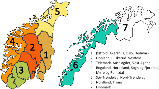
Fig. 1. Norwegian forest inventory (NFI) regions. The analyses cover region 1 through 6. Region 7 is excluded from the analyses due to lack of data. The names of the counties comprising each region in the study period are shown to the right.
| Table 1. Descriptive statistics of forest and forestry conditions in the six regions covered by the analyses. Data is from the middle of the study period (1996–2016). Source: Statistics Norway (2018b); Statistics Norway (2018d); Statistics Norway (2018e); Statistics Norway (2018f); Statistics Norway (2018g). | |||||||
| Region/Counties1 | Forest area, km2 | Growing stock, Mm3 | Share mature forest | Annual harvest, 1000 m3 | Average property size, ha | Harvest intensity, m3 ha–1 | |
| All | 79 955 | 746 | 38% | 7801 | 68 | 1.0 | |
| 1 | Østfold, Akershus, Oslo, Hedmark | 19 718 | 211 | 30% | 3384 | 93 | 1.7 |
| 2 | Oppland, Buskerud, Vestfold | 15 430 | 158 | 36% | 2280 | 72 | 1.5 |
| 3 | Telemark, Aust-Agder, Vest-Agder | 11 923 | 131 | 43% | 1024 | 74 | 0.9 |
| 4 | Rogaland, Hordaland, Sogn og Fjordane, Møre og Romsdal | 10 552 | 106 | 40% | 268 | 39 | 0.3 |
| 5 | Sør-Trøndelag, Nord-Trøndelag | 10 901 | 86 | 40% | 717 | 81 | 0.7 |
| 6 | Nordland, Troms | 11 432 | 54 | 47% | 128 | 63 | 0.1 |
| 1 As of January 1, 2020 some of the counties were merged in a regional reform. Some of the counties in regions 1–3 were merged across regions. The regions are so far not adjusted in the NFI data as reported by Statistics Norway. | |||||||
As we see from the table, there are rather larger differences between the regions regarding average harvest intensity and holding size. The inland regions (region 1 and 2) have a higher harvest intensity and a lower share of mature forest. Region 4 (Western Norway) and region 6 (Northern Norway) have the lowest harvest intensities. Parts of the country, especially along the coast, were planted with spruce (Norway spruce and to some extent Sitka spruce that both are non-native species there) replacing pine, broadleaves and other species with lower production. This activity peaked in the 1960ies and 1970ies. Thus, in parts of the country “modern” forestry is relatively new, and this together with the differences mentioned above, might be important for the main topic in this study.
The data on harvest and prices from Statistics Norway are divided into 16 assortments (7 for spruce and pine and 2 for broad-leaved species). In this study we have not differentiated between the species, and we have aggregated the 16 assortments to two: sawlogs and pulpwood. Prices used are volume weighted average prices for the underlying assortments for the two main types of timber. Fig. 2 shows the total harvest in the different regions over the time period analyzed.
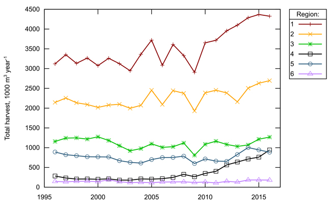
Fig. 2. Total industrial harvest in the six regions for which the analyses cover, 1000 m3 year–1. Source: Statistics Norway (2018b).
The total harvest is stable up to about 2010 and show an increasing trend thereafter. For some of the regions (1–3) there seem to be an increasing variation in harvest between years. It is noteworthy that region 4 shows a strong positive trend (in relative terms) in the last half of the analysis period.
Prices are deflated to 2016 level by using the consumer price index (Statistics Norway 2018a) and are shown in Supplementary file S1. We see a downward trend in both sawlog and pulpwood prices, as well as regional differences. In general, the prices are higher in the two inland regions compared to those along the western coast. We think this is due to tree species and assortment/quality composition that vary between regions.
For the interest rate we use the average interest on loans offered from Norwegian banks adjusted for inflation (Statistics Norway 2018a, 2018h), i.e., the real interest rate (Suppl. file S2).
Table 2 shows the correlation between the variables (in non-transformed form) used in the analyses.
| Table 2. Correlation (Pearson correlation coefficient) between variables used in the timber supply analyses. Variables are not transformed (i.e. not in log-form). | ||||||
| Sawlog harvest | Pulpwood harvest | Sawlog price | Pulpwood price | Standing stock | Interest rate | |
| Sawlog harvest | 1.00 | 0.97 | 0.36 | –0.07 | 0.93 | –0.08 |
| Pulpwood harvest | 0.97 | 1.00 | 0.36 | –0.03 | 0.92 | –0.08 |
| Sawlog price | 0.36 | 0.36 | 1.00 | 0.73 | 0.16 | 0.50 |
| Pulpwood price | –0.07 | –0.03 | 0.73 | 1.00 | –0.25 | 0.72 |
| Standing stock | 0.93 | 0.92 | 0.16 | –0.25 | 1.00 | –0.20 |
| Interest rate | –0.08 | –0.08 | 0.50 | 0.72 | –0.20 | 1.00 |
2.2 Theoretical model
The theoretical model applied in this study for justifying the choice of dependent and independent variables is adapted from Bolkesjø et al. (2010). Similar models have been used, see e.g. Binkley (1981); Kuuluvainen and Salo (1991); Prestemon and Wear (2000); Amacher et al. (2003); Amacher et al. (2009). The model assumes that forest owners operate in a competitive environment and maximize yearly profit conditional on current level of growing stock. Their short run optimization problem is thus:
![]()
subject to:
![]()
where π is the short term profit, R(•) is gross income from harvest as a function of sawlog quantity harvested (qs), sawlog price (ps), pulpwood quantity harvested (qm), and pulpwood price (pm). C(•) is the production cost as a function of standing stock (v), interest rate (r) and the harvested quantity of the two timber assortments. The standing stock may be used to produce different combinations of sawlog and pulpwood according to the implicit transformation frontier, g(•).
Assuming an unrestricted Cobb-Douglas functional form, the solution to the above optimization problem leads to the following short-term supply function:
![]()
where k and j refers to assortment (j ≠ k and with the following values: s = sawlog, m = pulpwood), αk is a constant, βk is the own price elasticity, βj is the cross price elasticity, γk is volume elasticity, δk is the elasticity with respect to the interest rate and e is the base of natural logarithms. Cobb-Douglas models have previously been applied in timber supply modelling by e.g. Kallio et al. (1987); Beach et al. (2005); Turner et al. (2006); Morland et al. (2018), and have some basic properties suitable for our purpose like being flexible and having aggregation properties that means that we can go from the single forest owner model to regional timber supply (Brown 2017).
For comparison we have also estimated models for total harvest, i.e. not divided into the two main timber assortments. The results for the total harvest models are given in the Suppl. files S5 and S6, but we do not comment extensively on them.
Regarding hypothesis, these are also taken from Bolkesjø et al. (2010): positive own-price elasticities (βk > 0), positive or negative cross-price elasticities (βj ![]() 0), depending on whether sawlogs and pulpwood are complements or substitutes in production, positive volume elasticity (γk > 0), and positive interest rate effect (δk > 0). These hypotheses are consistent with hypotheses derived from a two-period Fisherian savings-consumption model with perfect capital markets (Kuuluvainen and Salo 1991). With credit rationing the own-price effect is ambiguous and the interest rate effect is negative.
0), depending on whether sawlogs and pulpwood are complements or substitutes in production, positive volume elasticity (γk > 0), and positive interest rate effect (δk > 0). These hypotheses are consistent with hypotheses derived from a two-period Fisherian savings-consumption model with perfect capital markets (Kuuluvainen and Salo 1991). With credit rationing the own-price effect is ambiguous and the interest rate effect is negative.
2.3 Econometric methods
2.3.1 Supply models
In order to investigate the importance of the choice of statistical method, we have used three main statistical methods: two one-way panel data methods (fixed and random effects) and the first difference method. For fixed-effects models, OLS estimation is used. Random-effects models use a two-stage approach. In the first stage, variance components are calculated, and these are used to standardize the data. In the second stage OLS regression is performed on the standardized data. The first difference models are estimated using OLS. We have also estimated dynamic versions of the three main methods, i.e. containing the lagged dependent variable, using the instrument variable method (generalized method of moments) of Arellano and Bond (1991). All models are estimated using PROC MODEL in SAS 9.2 for Windows (SAS Institute Inc 2008). Heteroscedasticity-corrected covariance matrices are used, but tests show few and small differences compared to the ordinary estimator.
Taking the log of both sides of the supply equation above and adding an error term give:
![]()
where ln(•) is the natural logarithm, k and j refers to assortment (j ≠ k and with the following values: s = sawlog, m = pulpwood), i refers to region (1–6), t refers to year (1996–2016), εkit is residual error and the rest of the terms as previously defined. This general specification is labeled static in the following.
In line with Bolkesjø et al. (2010) we also estimate dynamic supply functions, i.e.:
![]()
where qkit–1 is the harvest the previous year, and the rest of the terms are as defined above.
To emphasize the main theme of the paper we use regional dummies to investigate regional differences in own-price elasticities.
The one-way panel data methods assume that the residual error can be decomposed as follows:
![]()
where eki is a region-specific error term and ukit is remaining error. In the fixed effects models the first term is assumed to be constant over time controlling for region specific unobserved factors affecting harvest. The eki in the fixed effects models can thus be viewed as region specific intercept terms, and the models are therefore estimated without a common intercept term. In the random effects method eki is a random variable uncorrelated with the explanatory variables. The major difference between the estimation methods is therefore the assumption about the region-specific error term, eki: for random effects models E[eki] = 0, and for fixed effects models eki is constant (fixed).
One way to eliminate the region-specific error terms (eki) is to use the year-to-year differences in the variables rather than their levels. This result in the following supply equation specification (based on Eq. 4):
![]()
where Δ indicates first difference, e.g. ![]() This model is also estimated with region specific own price elasticities.
This model is also estimated with region specific own price elasticities.
By using seemingly unrelated regression (SUR, estimated using PROC SYSLIN in SAS (SAS Institute Inc 2008)), we simultaneously estimate sawlog and pulpwood supply functions. Sawlogs and pulpwood are jointly produced from the same tree. It is in principle possible to produce only pulpwood. Since the value of sawlogs are roughly twice that of pulpwood (Suppl. file S1), this will in practice only happen in thinnings and under very special circumstances. Low-grade sawlogs may, for example, be declassified into pulpwood. Due to quality requirements, it is in practice not possible to produce only sawlogs. According to the Norwegian Agriculture Agency (2018), sales of sawlogs constituted about 70% of the gross timber income for Norwegian forest owners in 2016, while accounting for about 50% of the volume harvested.
The SUR models are estimated with regional own price and volume elasticities, with the restriction that the volume elasticities and the effect of interest rate are required to be equal for both assortments. We use first differenced data to estimate the SUR model, and the total growing stock in the region is used as independent variable in both the sawlog and pulpwood supply estimations.
2.3.2 Specification test
Various tests exist for testing the assumptions about the error structure. The null hypothesis that all regional effects (eki) are equal in the fixed effects models is tested by using a fixed effects F-test (Greene 1993). This is essentially a test of whether the fixed effects model performs better than the pooled counterpart.
For testing the random effects assumption we use the Breusch-Pagan test (Breusch and Pagan 1980) and Hausman test (Hausman 1978). We have tested for autocorrelation by using the Breusch-Godfrey LM test (Breusch and Godfrey 1981; Baltagi and Li 1995). In the presence of autocorrelation OLS is inefficient, but for the static models above it is still consistent and unbiased. If the regression contains lagged dependent variable – i.e. the dynamic models – OLS will be both biased and inconsistent when residuals are autocorrelated (Greene 1993). We estimate the dynamic models with the Arellano and Bond (1991) estimator, and thus, autocorrelation will not be a major issue for those models.
A well-known problem when using time-series data is the non-stationary or existence of unit roots. If variables are non-stationary, tests are biased toward the rejection of the null hypothesis even in the case where the time series are independent random walks (Granger and Newbold 1974; Phillips 1986). The data in levels are non-stationary, while first difference data are stationary. If the non-stationary variables are cointegrated (Engle and Granger 1987) we can still estimate the long-run relationship between the dependent and independent variables. We have used the t-barN/T statistics in Im et al. (2003) to test the residuals from the OLS models (fixed effects models) for stationarity, i.e. cointegration. This test is denoted IPS-ADF below. This test applies only to static fixed effects models.
Finally, the models with region specific elastisities are tested against their “pooled” counterparts using a poolability F-test, i.e. a test that the regional price coefficients (βki) all are equal to the coefficient in the model with a common price elasticity (βk). This test is the same test as the fixed effects F-test mentioned above, but with different pairs of models. For each of the models with regional elasticities we have also tested these against each other (i.e. βki = βkl) using a Wald test. The results from these Wald tests are not shown.
3 Results
3.1 Fit and specification tests
The fixed effects F-tests show (Suppl. files S3–S5) that accounting for regional differences in the intercept term leads to models with significantly better fit. This holds in all cases at 1% level.
The Breusch-Pagan test results show that the degree of autocorrelation is lowest for the fixed effects models. The random effects models perform as the fixed effects models in terms of RMSE. The null hypothesis of the Hausman tests is not rejected in most cases – meaning that the random effects model is both consistent and efficient, while the fixed effects model is consistent but inefficient. On the other hand, we cannot reject the null hypothesis of the Breusch-Pagan test in most cases, meaning that the fixed effects models are appropriate. The autocorrelation is, however, more severe for the random effects models than the fixed effects models. The IPS-ADF test indicates that the time series are not cointegrated for the dynamic fixed effects model.
Suppl. files S3 and S4 show that that the first difference models perform well compared to the other specifications. This comes at the expense of two things: we are only partially able to check for regional effects since this is factored out, and the elasticities are short-term elasticities. We see a similar effect when comparing the static and dynamic versions of the models. The use of the lagged dependent variable reduces autocorrelation, but again, the estimated elasticities are short-term.
One important test regarding regional differences is the poolability test. This is a test whether the common slope model yields a better fit than the model with region specific slopes. The null hypothesis that there is no difference between regions regarding own price elasticity is rejected in all cases except for the first difference models (Table 3). Suppl. files S3 and S4 show a reduction in RMSE for the panel data methods when going from common slope to regional slopes assumptions, but for the first difference models we see a small increase.
| Table 3. Poolability F-tests (F-value and significance level) of timber supply models with regional own price elasticities. The null hypothesis is that all regional price elasticities are equal within each model. | |||
| Fixed effect | Random effect | First difference | |
| Pulpwood | |||
| Static | 7.2*** | 7.4*** | 0.9 |
| Dynamic | 2.9** | 4.7*** | 1.3 |
| Sawlogs | |||
| Static | 21.8*** | 21.9*** | 0.6 |
| Dynamic | 5.3*** | 4.9*** | 0.8 |
| Significance levels: *** = 1%, ** = 5%, * = 10% | |||
3.2 Parameter estimates
The parameter estimates with accompanying standard errors and significance levels are shown in Table 4 and Table 5 for pulpwood and sawlogs models, respectively. We first look at the pulpwood models.
| Table 4. Parameter estimates, standard errors (in parenthesis), and significance level indicators for pulpwood supply models. | |||
| Model | Fixed effect | Random effect | First difference |
| Static, common slope | |||
| Intercept | –6.20 (5.11) | ||
| Pulpwood price | 0.53 (0.37) | 0.58 (0.34)* | 0.50 (0.19)*** |
| Sawlog price | 0.04 (0.23) | 0.15 (0.25) | 0.04 (0.13) |
| Standing stock | 1.05 (0.53)** | 1.28 (0.38)*** | 0.85 (0.27)*** |
| Rate of return | –2.05 (1.07)* | –1.71 (1.36) | –0.39 (0.94) |
| Dynamic, common slope | |||
| Intercept | –4.38 (1.10)*** | ||
| Pulpwood price | 0.24 (0.14) | 0.15 (0.15) | 0.53(0.21)** |
| Sawlog price | 0.27 (0.10)*** | 0.11 (0.08) | 0.17(0.16) |
| Standing stock | 0.86 (0.20)*** | 0.45 (0.04)*** | –0.03(0.72) |
| Rate of return | –0.53 (0.79) | –1.28 (0.85) | –0.88(1.32) |
| Pulpwood harvest, t–1 | 0.81 (0.04)*** | 0.82 (0.03)*** | –0.08(0.07) |
| Static, regional slopes | |||
| Intercept | 1.57 (6.28) | ||
| Pulpwood price, region 1 | 0.04 (0.38) | 0.14 (0.36) | 0.30 (0.07)*** |
| Pulpwood price, region 2 | 0.53 (0.35) | 0.53 (0.34) | 0.57 (0.07)*** |
| Pulpwood price, region 3 | 1.59 (0.44)*** | 1.45 (0.42)*** | 1.00 (0.06)*** |
| Pulpwood price, region 4 | –0.35 (0.57) | –0.26 (0.54) | 0.52 (0.12)*** |
| Pulpwood price, region 5 | 0.35 (0.39) | 0.37 (0.38) | 0.23 (0.10)** |
| Pulpwood price, region 6 | 0.96 (0.56)* | 0.85 (0.53) | 0.13 (0.12) |
| Sawlog price | –0.22 (0.33) | –0.18 (0.31) | 0.02 (0.13) |
| Standing stock | 0.79 (0.46)* | 0.83 (0.46)* | 0.82 (0.31)*** |
| Rate of return | –2.34 (1.13)** | –2.27 (1.14)** | –0.19 (0.99) |
| Dynamic, regional slopes | |||
| Intercept | –8.45 (3.41)** | ||
| Pulpwood price, region 1 | 0.20 (0.12) | 0.21 (0.11)* | 0.44(0.13)*** |
| Pulpwood price, region 2 | 0.26 (0.08)*** | 0.26 (0.08)*** | 0.59(0.1)*** |
| Pulpwood price, region 3 | 0.77 (0.09)*** | 0.67 (0.09)*** | 1.05(0.15)*** |
| Pulpwood price, region 4 | –0.16 (0.23) | –0.08 (0.20) | 0.52(0.14)*** |
| Pulpwood price, region 5 | 0.04 (0.11) | 0.08 (0.11) | 0.24(0.26) |
| Pulpwood price, region 6 | 0.39 (0.13)*** | 0.36 (0.13)*** | 0.11(0.31) |
| Sawlog price | 0.17 (0.10)* | 0.19 (0.09)** | 0.13(0.17) |
| Standing stock | 0.81 (0.19)*** | 0.82 (0.20)*** | –0.53(0.83) |
| Rate of return | –0.74 (0.70) | –0.71 (0.71) | –0.65(1.38) |
| Pulpwood harvest, t–1 | 0.70 (0.07)*** | 0.72 (0.06)*** | –0.08(0.1) |
| Significance levels: *** = 1%, ** = 5%, * = 10% | |||
Given the standard errors of the estimates, there are rather small differences between the results of the fixed and random effects models. Comparing the estimates from the first difference model with the dynamic fixed and random effects models, we see that there are differences, but they are not very large. The volume elasticity (for total standing stock) is, given the standard errors of the estimates, very similar across all models. Thus, regarding this variable there seems to be some robustness with respect to model specification.
Most of the significant parameters have the sign as hypothesized, but it is noteworthy that the pulpwood price is significant in only about half the cases. Although not statistically significant, the price elasticity for region 4 (Western Norway) is negative for the fixed and random effects models. This is also the case for the sawlog models, and we will discuss this below.
Another exception is the rate of return. This variable is significantly positive only for sawlog fixed and random effects models (Table 5) and has a negative sign in all other models, although insignificantly different from zero for about two thirds of these models. We have tested different specifications for the interest rate variable. This include treating the interest rate as the other variables, i.e. estimating interest rate elasticities. The results from these alternative specifications are similar to the ones presented here regarding sign and significance level. We have also run models without the interest rate. Parameter estimates and standard errors remain remarkable similar and the 95% confidence intervals for the parameters are in all cases overlapping.
The differences in estimated elasticities between regions are for the most parts statistically significant at 5% or better (between 12 and 15 out of 15 pairs) according to the Wald test performed (not shown). Recall, however, that for the first difference models, the models with a common price elasticity perform slightly better (see the RMSE in Suppl. files S3 and S4 ). Certainly, if the estimates are to be used in a regionalized model, the pooled model with only one elasticity will be less accurate for the dynamics at the regional level.
If we turn to the sawlog model, we see much of the same pattern as for pulpwood regarding robustness (Table 5). The fixed and random effects models with regional own price elasticities result in negative elasticities for region 4 (along the western coast) – like for the pulpwood models as mentioned above. We also see this for the total harvest models shown in the Suppl. file S6. These results are contradictory to the theory presented above.
| Table 5. Parameter estimates, standard errors (in parenthesis), and significance level indicators for sawlog supply models. | |||
| Model | Fixed effect | Random effect | First difference |
| Static, common slope | |||
| Intercept | –11.14 (4.20)*** | ||
| Pulpwood price | –0.32 (0.27) | –0.27 (0.23) | 0.02 (0.14) |
| Sawlog price | 0.76 (0.23)*** | 0.88 (0.30)*** | 1.24 (0.13)*** |
| Standing stock | 1.50 (0.58)** | 1.73 (0.41)*** | 2.09 (0.32)*** |
| Rate of return | 1.60 (0.77)** | 1.95 (0.99)* | –1.44 (0.78)* |
| Dynamic, common slope | |||
| Intercept | –4.22 (2.03)** | ||
| Pulpwood price | –0.30 (0.15)* | –0.36 (0.09)*** | 0.23(0.15) |
| Sawlog price | 0.76 (0.13)*** | 0.64 (0.26)** | 1.01(0.08)*** |
| Standing stock | 0.75 (0.12)*** | 0.41 (0.17)** | 2.22(0.65)*** |
| Rate of return | 0.47 (0.63) | –0.17 (0.68) | –0.58(0.81) |
| Sawlog harvest, t–1 | 0.78 (0.16)*** | 0.82 (0.08)*** | –0.31(0.09)*** |
| Static, regional slopes | |||
| Intercept | 5.83 (1.65)*** | ||
| Pulpwood price | –0.57 (0.17)*** | –0.56 (0.18)*** | 0.04 (0.13) |
| Sawlog price, region 1 | 0.79 (0.09)*** | 0.79 (0.09)*** | 1.04 (0.03)*** |
| Sawlog price, region 2 | 0.72 (0.10)*** | 0.72 (0.11)*** | 1.30 (0.05)*** |
| Sawlog price, region 3 | 0.98 (0.12)*** | 0.97 (0.11)*** | 1.21 (0.04)*** |
| Sawlog price, region 4 | –2.67 (0.21)*** | –2.49 (0.19)*** | 0.74 (0.08)*** |
| Sawlog price, region 5 | 1.62 (0.12)*** | 1.57 (0.12)*** | 1.20 (0.04)*** |
| Sawlog price, region 6 | 0.53 (0.12)*** | 0.54 (0.12)*** | 1.77 (0.04)*** |
| Standing stock | 0.64 (0.24)*** | 0.69 (0.26)*** | 2.09 (0.31)*** |
| Rate of return | 1.03 (0.81) | 1.06 (0.81) | –1.45 (0.79)* |
| Dynamic, regional slopes | |||
| Intercept | –3.02 (3.67) | ||
| Pulpwood price | –0.47 (0.18)*** | –0.42 (0.18)** | 0.19(0.16) |
| Sawlog price, region 1 | 0.78 (0.07)*** | 0.76 (0.08)*** | 0.88(0.09)*** |
| Sawlog price, region 2 | 0.80 (0.07)*** | 0.78 (0.08)*** | 1.07(0.12)*** |
| Sawlog price, region 3 | 0.95 (0.09)*** | 0.91 (0.10)*** | 0.76(0.25)*** |
| Sawlog price, region 4 | –1.26 (0.68)* | –0.75 (0.56) | 0.81(0.14)*** |
| Sawlog price, region 5 | 1.19 (0.20)*** | 1.06 (0.20)*** | 0.94(0.21)*** |
| Sawlog price, region 6 | 0.76 (0.10)*** | 0.77 (0.08)*** | 1.72(0.15)*** |
| Standing stock | 0.59 (0.16)*** | 0.63 (0.15)*** | 2.11(0.63)*** |
| Rate of return | 0.73 (0.64) | 0.66 (0.63) | –0.85(0.77) |
| Sawlog harvest, t–1 | 0.50 (0.18)*** | 0.57 (0.19)*** | –0.30(0.1)*** |
| Significance levels: *** = 1%, ** = 5%, * = 10% | |||
Table 6 shows the parameter estimates, standard errors and significance level of the SUR model along with the corresponding unconstrained OLS models. The latter are comparable to the first difference static models with regional slopes presented in Table 4 and Table 5. Fit statistics for the SUR are acceptable, but far from impressive (r2 = 0.28 and RMSE = 0.14). Price elasticities for the OLS models are close to the ones presented above, i.e. for models with a common standing stock elasticity.
| Table 6. Unconstrained OLS and seemingly unrelated regression (SUR) pulpwood and sawlog supply models. Parameter estimates, standard errors (in parenthesis), and significance level indicators for first difference models. | ||||
| Elasticity | Pulpwood | Sawlog | ||
| Unconstrained OLS | Constrained SUR | Unconstrained OLS | Constrained SUR | |
| Own price, region 1 | 0.35 (0.34) | 0.30 (0.30) | 1.02 (0.36)*** | 0.90 (0.33)*** |
| Own price, region 2 | 0.61 (0.35)* | 0.50 (0.31) | 1.32 (0.38)*** | 1.21 (0.35)*** |
| Own price, region 3 | 1.00 (0.33)*** | 0.96 (0.30)*** | 1.21 (0.38)*** | 1.30 (0.34)*** |
| Own price, region 4 | 0.58 (0.37) | 0.79 (0.33)** | 0.80 (0.55) | 0.88 (0.50)* |
| Own price, region 5 | 0.16 (0.38) | 0.34 (0.33) | 1.12 (0.42)** | 0.97 (0.39)** |
| Own price, region 6 | 0.02 (0.40) | 0.46 (0.37) | 1.83 (0.42)*** | 1.85 (0.38)*** |
| Cross price | 0.01 (0.17) | 0.05 (0.17) | 0.03 (0.18) | –0.06 (0.17) |
| Standing stock, region 1 | 1.77 (1.90) | 1.39 (1.65) | 1.25 (1.97) | 1.39 (1.65) |
| Standing stock, region 2 | 1.73 (2.37) | 1.84 (2.05) | 2.66 (2.40) | 1.84 (2.05) |
| Standing stock, region 3 | 0.83 (1.52) | 1.29 (1.32) | 1.98 (0.59) | 1.29 (1.32) |
| Standing stock, region 4 | 1.24 (1.05) | 1.86 (0.91)** | 2.40 (1.09)** | 1.86 (0.91)** |
| Standing stock, region 5 | 0.02 (1.19) | 0.36 (1.44) | 0.66 (1.71) | 0.36 (1.44) |
| Standing stock, region 6 | –0.19 (0.95) | 1.42 (1.19) | 2.86 (1.43)** | 1.42 (1.19) |
| Rate of return | –0.16 (1.01) | –0.83 (0.84) | –1.46 (1.04) | –0.83 (0.84) |
| Significance levels: *** = 1%, ** = 5%, * = 10% | ||||
The price elasticities, especially for sawlogs, are of the same magnitude in both the unconstrained (OLS) and constrained (SUR) models. This is in contrast to the volume elasticities where there are large differences. For the SUR sawlog model, all own price elasticities are significant at 10% level or better, while for pulpwood only two (for region 3 and 4) are significantly different from zero and only region 4 has a significant volume elasticity. There are few differences in elasticities across regions (tests not shown); the sawlog price elasticity in region 1 is significantly different (at 5% level) from region 6, and this elasticity for region 5 is different from region 6 (at 10% level). The cross-price elasticities are small and not significant. This is in line with the results of the first difference models presented earlier. Only the restrictions on the standing stock elasticity for region 6 is significant (at 5% level).
4 Discussion
The specification tests show that the first difference models are overall the best for estimating short-term elasticities. These models also give results which are in accordance with economic theory. First difference models with region-specific price parameters do not perform significantly better in terms of fit than models with a common price parameter. In the regionalized models, regional prices are for a large part significant, especially for sawlog models, and according to Wald tests the parameters are significantly different. They will give more accurate regional estimates, although the overall fit will be about the same. If regionalization is important, we recommend using the SUR approach to enhance consistency between sawlog and pulpwood supply – after carefully checking and testing separate econometric specification in order to avoid for example spurious regressions.
The results show clear differences between the regions regarding timber supply, and that the approaches used here perform well in most cases. The region along the western coast (region 4) stands out as quite different from the other regions. Here the harvest has been monotonically increasing despite a negative trend in real timber prices. The panel data methods give negative price elasticities in region 4, while short-term price elasticities estimated using first difference models are all positive. The former is not in line with economic theory and could in our opinion be caused by structural factors special for this region, as discussed below.
The fixed and random effects models give rather similar results. Based on the nature of the data, one could easily argue for the use of fixed effects models, as the differences in “intercept” terms between the regions are clearly visible in Fig. 2. On the other hand, the division into NFI regions is probably based on the conditions for forest production and forestry, but with respect to timber supply, the division must be said to be more or less random. There are therefore arguments supporting also the random effects approach.
From a statistical point of view, the choice between the random and fixed effects model is also to some degree a choice between inefficiency and bias (Clark and Linzer 2015). If parameter values matter, e.g. regional price elasticities for the use in forest sector models, then fixed effects models would in general be better since the regional aspects would be clearer. In addition, the choice of specification should not be guided by statistical properties only. In our case, there is a larger across than within variation in harvest levels (see Fig. 2). This could justify the use of a fixed effects model, but would not rule out a random effects model, per se.
First difference and dynamic models removes the potential problems from non-stationarity. This is as expected. Elasticities estimated by these models are short-term whereas the estimated static models give long-term elasticities. For sawlog models, static and dynamic own price elasticities are practically equal and in general lower than for the first difference models. This means that forest owners respond to prices more in the short than the long term. One possible explanation to this is that income from harvests is not very important for the major part of owners, and that they therefore can take advantage of price increases.
It is not easy to explain the result reported in section 3 that the interest rate is significantly positive only in the static sawlog fixed and random effects models with common slope, and otherwise negative and mostly non-significant. One reason could be that there are rather strong correlations between the three variables interest rate, sawlog price and pulpwood price as shown in Table 2, and that the price variables capture the interest rate effect.
The supply elasticities estimated in the Norwegian studies mentioned in section 1 differ much, from 0.53 to 1.54 for wood price; from 0.10 to 0.78 for standing forest volume, and from zero to 0.28 for real interest rate before tax. In addition to differences regarding the choice of dependent and independent variables, many factors, like econometric method used, functional form assumed, data quality and sample selection (size, period, aggregation level, etc), are likely reasons for the rather large variations obtained. Bolkesjø et al. (2010) show somewhat lower own price and volume elasticities for sawlogs for a comparable first difference model. For pulpwood the own price elasticities are almost identical, while our volume elasticities are much lower.
Region 4 – along the western coast – appears to have a different dynamic compared to the other regions. Here the harvest has been monotonically increasing despite a negative trend in real timber prices. The models estimating long-term elasticities, i.e. the static fixed and random effects models, yield negative price elasticities in region 4 while the first difference models yield positive elasticities. This implies that forest owners react to short term variation in prices, but that there are underlying long term changes not captured by our models. It is beyond the scope of this paper to investigate the seemingly atypical harvest behavior in region 4 in detail, but some explanations can be hypothesized.
The largest increase in harvest in region 4 was between 2011 and 2012. The main explanation to this is the hurricane Dagmar that hit the western coast on December 25, 2011. The harvest in Sogn og Fjordane County (the second county from north in this region, ref. Fig. 1) increased by almost 200% from 2011 to 2012. The harvest in Møre og Romsdal County increased by 40%. The effects in the two last counties in this region were negligible.
In region 4 as a whole, the standing stock increased by 55% (Statistics Norway 2018e) and the share of mature forest, i.e. in maturity class V, increased by 42% (Statistics Norway 2018d) in the period investigated. The corresponding figures for the whole of Norway are 36% and 21%, respectively. Also, during the period covered by the study, this region has been influenced by several other factors that might have impacted the timber supply, like changes in timber buyers’ activities and subsidies for logging operations, road and harbor constructions and road transport.
Underlying structural changes not included in the data are more likely causes for the harvest increase than single events. The importance of these factors should be investigated in future analyses. It is important to note that the first difference models capture the short term reactions to price changes in a way that is consistent with economic theory, i.e. giving positive price elasticities. This underlines that careful testing of econometric specifications is necessary.
5 Conclusions
The main aim of this study is to analyze and quantify the Norwegian timber supply at regional level, having as the main hypothesis that there are differences between regions. The specification tests show that the first difference models perform better than the fixed effects and random effects panel models used in the study. The first difference models give estimates of short-term elasticities.
Models with region-specific price parameters do not perform much better in terms of overall fit than models with a common price parameter – although the difference is statistically significant for the fixed and random effects models. In the regionalized models, regional prices are for a large part significant, especially for sawlog models, and the price parameters are significantly different. Such models will perform better at the regional level although the overall national fit will be about the same. If regionalization is important, we recommend using a SUR approach to enhance consistency between sawlog and pulpwood supply – after carefully checking and testing separate econometric specification in order to avoid for example spurious regressions.
The two panel models estimating long-term elasticities give negative price elasticities in region 4, while short-term price elasticities estimated using first difference models are all positive. The former is not in line with economic theory and could in our opinion be caused by structural factors special for this region during the period covered by the study, like storm damages, changes in timber buyers’ activities, and subsidies for logging operations, road and harbor constructions and road transport. The impacts of such factors should be investigated in future analyses.
Funding and acknowledgement
This study was done in the following projects funded by the Research Council of Norway: SUPOENER: The Future Role of Biomass Energy in Norway (186946/i30), FME CenBio – Bioenergy Innovation Centre (212701) and FME Bio4Fuels – Norwegian Centre for Sustainable Bio-based Fuels and Energy (257622). We also thank three anonymous reviewers and the editors for comments and suggestions that have improved the paper.
Author contribution
Per Kristian Rørstad: Conceptualization, Methodology, Data Curation, Formal Analysis, Writing – Original Draft, Writing – Review and Editing, Erik Trømborg: Writing – Review and Editing, Supervision, Birger Solberg: Conceptualization, Writing – Review and Editing, Supervision, Project Administration, Funding Acquisition.
Declaration of openness of research materials and data
The main dataset used is compiled from open sources – see the references – and it is freely available upon request. The SAS code files used for the analyses presented in this study are also freely available upon request. Please send an email to the corresponding author.
References
Amacher GS, Conway MC, Sullivan J (2003) Econometric analyses of nonindustrial forest landowners: Is there anything left to study? J For Econ 9: 137–164. https://doi.org/10.1078/1104-6899-00028.
Amacher GS, Koskela E, Ollikainen M (2009) Economics of forest resources. The MIT Press, Cambridge, Mass.
Andrade IC (2000) Production technology in the pulp and paper industry in the European Union: factor substitution, economies of scale, and technological change. J For Econ 6: 23–39.
Arellano M, Bond S (1991) Some tests of specification for panel data: Monte Carlo evidence and an application to employment equations. Rev Econ Stud 58: 277–297. https://doi.org/10.2307/2297968.
Baardsen S, Nyrud AQ, Veidahl A (1997) Analyser av de norske tømmermarkedene. [Analyses of the Norwegian timber markets, in Norwegian]. In: Eid T, Hoen HF, Solberg B (eds) Meddelelser fra Skogforsk, Festskrift til ære for professorene John Eid, Sveinung Nersten, Asbjørn Svendsrud. [Festschrift in the honor of the professors John Eid, Sveinung Nersten, Asbjørn Svendsrud], pp. 17–44. Skogforsk, Ås.
Baltagi BH, Li Q (1995) Testing Ar(1) against Ma(1) disturbances in an error component model. J Econometrics 68: 133–151. https://doi.org/10.1016/0304-4076(94)01646-H.
Bashir A, Sjølie HK, Solberg B (2020) Determinants of nonindustrial private forest owners’ willingness to harvest timber in Norway. Forests 11, article id 60. https://doi.org/10.3390/f11010060.
Beach RH, Pattanayak SK, Yang J-C, Murray BC, Abt RC (2005) Econometric studies of non-industrial private forest management: a review and synthesis. Forest Pol Econ 7: 261–281. https://doi.org/10.1016/s1389-9341(03)00065-0.
Binkley CS (1981) Timber supply from private nonindustrial forests: a microeconomic analysis of landowner behavior. Yale School of the Environment Bulletin Series 7, vol. 92, Yale University, New Haven.
Binkley CS (1987) Economic models of timber supply. In: Kallio M, Dykstra DP, Binkley CS (eds) The Global forest sector: an analytical perspective, pp. 109–136. John Wiley and Sons, Chichester.
Bolkesjø TF, Baardsen S (2002) Roundwood supply in Norway: micro-level analysis of self-employed forest owners. Forest Pol Econ 4: 55–64. https://doi.org/10.1016/S1389-9341(01)00081-8.
Bolkesjø TF, Solberg B (2003) A panel data analysis of nonindustrial private roundwood supply with emphasis on the price elasticity. For Sci 49: 530–538.
Bolkesjø TF, Solberg B, Wangen KR (2007) Heterogeneity in nonindustrial private roundwood supply: lessons from a large panel of forest owners. J For Econ 13: 7–28. https://doi.org/10.1016/j.jfe.2006.08.003.
Bolkesjø TF, Buongiorno J, Solberg B (2010) Joint production and substitution in timber supply: a panel data analysis. Appl Econ 42: 671–680. https://doi.org/10.1080/00036840701721216.
Brännlund R, Johansson PO, Löfgren KG (1985) An econometric-analysis of aggregate sawtimber and pulpwood supply in Sweden. For Sci 31: 595–606.
Breusch TS, Godfrey LG (1981) A review of recent work on testing for autocorrelation in dynamic simultaneous models. In: Currie D, Nobay R, Peel D (eds) Macroeconomic analysis: essays in macroeconomics and econometrics, pp. 63–110. Croom Helm, London.
Breusch TS, Pagan AR (1980) The lagrange multiplier test and its applications to model-specification in econometrics. Rev Econ Stud 47: 239–253. https://doi.org/10.2307/2297111.
Brough P, Rørstad PK, Breland TA, Trømborg E (2013) Exploring Norwegian forest owner’s intentions to provide harvest resides for bioenergy. Biomass Bioenerg 57: 57–67. https://doi.org/10.1016/j.biombioe.2013.04.009.
Brown M (2017) Cobb–Douglas functions. In: The new Palgrave dictionary of economics, pp. 1–4. Palgrave Macmillan, London, UK. https://doi.org/10.1057/978-1-349-95121-5_480-2.
Camia A, Giuntoli J, Jonsson R, Robert N, Cazzaniga NE, Jasinevičius G, Avitabile V, Grassi G, Barredo JI, Mubareka S (2021) The use of woody biomass for energy purposes in the EU. Publications Office of the European Union, Luxembourg. https://data.europa.eu/doi/10.2760/428400.
CEPI (2020) Key statistics 2019 – European pulp and paper industry. The Confederation of European Paper Industries, Brussels, Belgum.
Clark TS, Linzer DA (2015) Should I use fixed or random effects? Political Sci Res Methods 3: 399–408. https://doi.org/doi:10.1017/psrm.2014.32.
de Jong W, Galloway G, Katila P, Pacheco P (2017) Forestry discourses and forest based development – an introduction to the Special Issue. Int For Rev 19: 1–9. https://doi.org/10.1505/146554817822407358.
Engle RF, Granger CWJ (1987) Cointegration and error correction – representation, estimation, and testing. Econometrica 55: 251–276. https://doi.org/10.2307/1913236.
FAO (2009) Pulp and paper capacities 2008–2013. Food and Agriculture Organization of the United Nations.
FAO (2016) Pulp and paper capacities 2015–2020. Food and Agriculture Organization of the United Nations.
Favada IM, Karppinen H, Kuuluvainen J, Mikkola J, Stavness C (2009) Effects of timber prices, ownership objectives, and owner characteristics on timber supply. For Sci 55: 512–523.
Forest Europe (2020) State of Europe’s forests 2020. Ministerial Conference on the Protection of Forests in Europe, Forest Europe Liaison Unit Bratislava.
Granger CWJ, Newbold P (1974) Spurious regressions in econometrics. J Econometrics 2: 111–120. https://doi.org/10.1016/0304-4076(74)90034-7.
Greene WH (1993) Econometric analysis, 2nd ed. Macmillan, New York.
Hausman JA (1978) Specification tests in econometrics. Econometrica 46: 1251–1271. https://doi.org/10.2307/1913827.
Hurmekoski E, Hetemäki L (2013) Studying the future of the forest sector: review and implications for long-term outlook studies. Forest Pol Econ 34: 17–29. https://doi.org/10.1016/j.forpol.2013.05.005.
Im KS, Pesaran MH, Shin Y (2003) Testing for unit roots in heterogeneous panels. J Econometrics, 115: 53–74. https://doi.org/10.1016/S0304-4076(03)00092-7.
Jåstad EO, Bolkesjø TF, Trømborg E, Rørstad PK (2019) Large-scale forest-based biofuel production in the Nordic forest sector: effects on the economics of forestry and forest industries. Energ Convers Manage 184: 374–388. https://doi.org/10.1016/j.enconman.2019.01.065.
Jåstad EO, Bolkesjø TF, Rørstad PK (2020) Modelling effects of policies for increased production of forest-based liquid biofuel in the Nordic countries. Forest Pol Econ 113, article id 102091. https://doi.org/10.1016/j.forpol.2020.102091.
Kallio AMI (2021) Wood-based textile fibre market as part of the global forest-based bioeconomy. Forest Pol Econ 123, article id 102364. https://doi.org/10.1016/j.forpol.2020.102364.
Kallio AMI, Solberg B, Käär L, Päivinen R (2018) Economic impacts of setting reference levels for the forest carbon sinks in the EU on the European forest sector. Forest Pol Econ 92: 193–201. https://doi.org/10.1016/j.forpol.2018.04.010.
Kallio M, Dykstra DP, Binkley CS (1987) The global forest sector: an analytical perspective. John Wiley and Sons Inc, New York, NY.
Kuuluvainen J, Salo J (1991) Timber supply and life-cycle harvest of nonindustrial private forest owners – an empirical analysis of the Finnish case. For Sci 37: 1011–1029.
Kuuluvainen J, Tahvonen O (1999) Testing the forest rotation model: evidence from panel data. For Sci 45: 539–551.
Kuuluvainen J, Favada IM, Uusivuori J (2006) Empirical behaviour models on timber supply. In: Aronsson T, Axelsson R, Brännlund R (eds) The theory and practice of environmental and resource economics: essays in honour of Karl-Gustaf Löfgren, pp. 225–245. Edward Elgar, Cheltenham.
Kuuluvainen J, Karppinen H, Hänninen H, Uusivuori J (2014) Effects of gender and length of land tenure on timber supply in Finland. J For Econ 20: 363–379. https://doi.org/10.1016/j.jfe.2014.10.002.
Latta GS, Plantinga AJ, Sloggy MR (2015) The effects of internet use on global demand for paper products. J Forest 114: 433–440. https://doi.org/10.5849/jof.15-096.
Løyland K, Ringstad V, Øy H (1995) Determinants of forest activities – a study of private nonindustrial forestry in Norway. J For Econ 1: 219–237.
Månsson J (2003) Economies of scale in the Swedish sawmill industry. J For Econ 9: 169–179. https://doi.org/10.1078/1104-6899-00033.
Morland C, Schier F, Janzen N, Weimar H (2018) Supply and demand functions for global wood markets: specification and plausibility testing of econometric models within the global forest sector. Forest Pol Econ 92: 92–105. https://doi.org/doi.org/10.1016/j.forpol.2018.04.003.
Norwegian Agriculture Agency (2018) Tømmeravvirkning og -priser. [Timber harvest and prices]. https://www.landbruksdirektoratet.no/nb/statistikk-og-utviklingstrekk/utviklingstrekk-i-skogbruket/tommeravvirkning-og-priser. Landbruksdirektoratet.
Phillips PCB (1986) Understanding spurious regressions in econometrics. J Econometrics 33: 311–340. https://doi.org/10.1016/0304-4076(86)90001-1.
Pingoud K, Pohjola J, Valsta L (2010) Assessing the integrated climatic impacts of forestry and wood products. Silva Fenn 44: 155–175. https://doi.org/10.14214/sf.166.
Polyakov M, Wear DN, Huggett RN (2010) Harvest choice and timber supply models for forest forecasting. For Sci 56: 344–355.
Prestemon JP, Wear DN (2000) Linking harvest choices to timber supply. For Sci 46: 377–389.
Rørstad PK (1990) Faktorer som påvirker tømmertilbudet fra private skogeiere – en økonometrisk analyse. [Factors affecting timber supply form private forest owner – an econometric analysis]. Cand agric thesis. Agricultural University of Norway, Ås.
Rørstad PK, Solberg B (1992) A Tobit analysis of the non-industrial private timber supply behaviour in Norway. In: Solberg B (ed) Proceedings of the biennial meeting of the scandinavian society of forest economics, Gausdal, Norway, April 1991. Scandinavian Forest Economics 33: 352–371.
SAS Institute Inc (2008) SAS/ETS 9.2 User’s guide. SAS Institute Inc., Cary, NC.
Sjølie HK, Becker D, Håbesland D, Solberg B, Lindstad BH, Snyder S, Kilgore M (2016) Willingness of nonindustrial private forest owners in Norway to supply logging residues for wood energy. Small-scale For 15: 29–43. https://doi.org/10.1007/s11842-015-9306-x.
Sjølie HK, Wangen KR, Lindstad BH, Solberg B (2019) The importance of timber prices and other factors for harvest increase among non-industrial private forest owners. Can J For Res, 49 (5): 543–552. https://doi.org/10.1139/cjfr-2018-0292.
Solberg B, Moiseyev A, Hansen JØ, Horn SJ, Øverland M (2021) Wood for food: economic impacts of sustainable use of forest biomass for salmon feed production in Norway. Forest Pol Econ 122, article id 102337. https://doi.org/10.1016/j.forpol.2020.102337.
Statistics Norway (2018a) StatBank Norway table 03014: consumer price index. https://www.ssb.no/en/statbank/table/03014. Accessed 15 March 2018.
Statistics Norway (2018b) StatBank Norway table 03895: commercial removals of industrial roundwood, by assortment (m3) (M). https://www.ssb.no/en/statbank/table/03895. Accessed 15 March 2018.
Statistics Norway (2018c) StatBank Norway table 06216: average price, by assortment (NOK per m3) (C). https://www.ssb.no/en/statbank/table/06216. Accessed 15 March 2018.
Statistics Norway (2018d) StatBank Norway table 06287: productive forest area, by development class, site quality and surveyed regions. Available at: https://www.ssb.no/en/statbank/table/06287. Accessed 15 March 2018.
Statistics Norway (2018e) StatBank Norway table 06290: growing stock under bark, by type of land, species of tree and surveyed regions (1000 m3). https://www.ssb.no/en/statbank/table/06290. Accessed 15 March 2018.
Statistics Norway (2018f) StatBank Norway table 06307: forest properties, by size class (decares) (C). https://www.ssb.no/en/statbank/table/06307. Accessed 15 March 2018.
Statistics Norway (2018g) StatBank Norway table 08198: total area, by type of vegetation and surveyed regions (km2). Available at: https://www.ssb.no/en/statbank/table/08198. Accessed 15 March 2018.
Statistics Norway (2018h) StatBank Norway table: 08175: yearly interest rates on loans and deposits. Complete census (per cent). https://www.ssb.no/en/statbank/table/08175. Accessed 15 March 2018.
Størdal S, Baardsen S (2003) An econometric analysis of differences in stumpage values using micro-level harvesting data. In: Helles F, Strange N, Wichmann L (eds) Recent accomplishments in applied forest economics research. For Sci 74: 63–71. Kluwer, Dordrecht. https://doi.org/10.1007/978-94-017-0279-9_5.
Størdal S, Lein K, Ørbeck M, Hagen S (2004) Regional differences in harvesting levels and wood-based employment in Norway. Small-scale For 3: 35–47. https://doi.org/10.1007/s11842-004-0003-4.
Størdal S, Lien G, Baardsen S (2008) Analyzing determinants of forest owners’ decision-making using a sample selection framework. J For Econ 14: 159–176. https://doi.org/10.1016/j.jfe.2007.07.001.
Trømborg E, Jåstad EO, Bolkesjø TF, Rørstad PK (2020) Prospects for the Norwegian forest sector: a green shift to come? J For Econ 35: 305–336. https://doi.org/10.1561/112.00000517.
Turner JA, Buongiorno J, Zhu S (2006) An economic model of international wood supply, forest stock and forest area change. Scan J For Res 21: 73–86. https://doi.org/10.1080/02827580500478506.
Vennesland B, Hobbelstad K, Bolkesjø T, Baardsen S, Lileng J, Rolstad J (2006) Skogressursene i Norge 2006 – muligheter og aktuelle strategierfor økt avvirkning. [Forest resources in Norway 2006 – possibilities and strategies for increased harvest]. Viten fra Skog og landskap 3/2006. The Norwegian Forest and Landscape Institute, Ås.
Total of 71 references.
