The effect of winter weather on timber truck tare weights
Anttila P., Nummelin T., Väätäinen K., Laitila J. (2020). The effect of winter weather on timber truck tare weights. Silva Fennica vol. 54 no. 4 article id 10385. https://doi.org/10.14214/sf.10385
Highlights
- In a one-year follow-up study of eight timber trucks in Finland, up to 6–12% increase in tare weights was observed in wintertime
- Compared with summertime tare weights, the maximum increase varied between 1560 kg and 3100 kg
- Potential payload loss was explained by temperature, relative humidity and precipitation.
Abstract
In wintertime, the payload capacity of a timber truck is reduced by snow that accumulates on the structures of the truck. The aim of this study was to quantify the potential payload loss due to snow and winter accessories and to predict the loss with weather variables. Tare weights of eight timber trucks were collected at mill receptions in Finland over a one-year period. Monthly and annual loss of potential payload was estimated using the tare measurements in summer months as a reference. Each load was also connected with weather data at the location and time of delivery and payload loss explained by the weather data with the aid of regression models. The maximum loss of payload varied between 1560 kg and 3100 kg. On a monthly basis, the highest losses occurred in January, when the median values varied between 760 kg and 2180 kg. Over the year, the payload loss ranged between the trucks from 0.5% to 1.5% (from 1.9% and 5.1% in January) of the total number of loads in the study. Payload loss was found to increase with decreasing temperature, increasing relative humidity and increasing precipitation. Although the average payload loss was not very high, the biggest losses occur just during the season of highest capacity utilization. Big differences were also found in the tare weights between the trucks. The results of the study give incentive to develop truck and trailer structures that reduce the adherence of snow.
Keywords
forestry logistics;
payload;
tare weight;
weather data
-
Anttila,
Natural Resources Institute Finland (Luke), Latokartanonkaari 9, FI-00790 Helsinki, Finland
 https://orcid.org/0000-0002-6131-392X
E-mail
perttu.anttila@luke.fi

- Nummelin, Natural Resources Institute Finland (Luke), Latokartanonkaari 9, FI-00790 Helsinki, Finland E-mail tuomas.nummelin@luke.fi
- Väätäinen, Natural Resources Institute Finland (Luke), Yliopistokatu 6, FI-80100 Joensuu, Finland E-mail kari.vaatainen@luke.fi
-
Laitila,
Natural Resources Institute Finland (Luke), Yliopistokatu 6, FI-80100 Joensuu, Finland
 https://orcid.org/0000-0003-4431-3319
E-mail
juha.laitila@luke.fi
Received 26 May 2020 Accepted 17 September 2020 Published 21 September 2020
Views 45170
Available at https://doi.org/10.14214/sf.10385 | Download PDF

1 Introduction
Timber logistics relies heavily on road transport. In Finland, for instance, over 76% of timber transported in 2018 was carried by truck (most often a truck and trailer combination) (Strandström 2019). Even if other transport modes were used, at least the first leg of the trip is done by truck. Considering the importance of truck transport, it is natural that a lot of effort has been directed to its research and development – especially in order to minimize transport costs and greenhouse gas emissions. Savings can be achieved by optimizing timber flows and transport routes (Rönnqvist 2003) or by improving the condition and maintenance of roads (Malinen et al. 2014). By increasing Gross Vehicle Weight (GVW) and dimensions of load space, the costs and emissions per transported tonne can be decreased (Laitila et al. 2016; Palander 2016; Palander 2017; Asmoarp et al. 2018; Venäläinen and Poikela 2019; Väätäinen et al. 2020).
Yet another way to increase payloads is to minimize the weight of an empty truck, i.e. the tare weight. According to Erlandsson (2008) the net margin of a trucking company increased, on average, by almost five percentage units when the fleet’s average tare weight decreased by one tonne. Shaffer and Stuart (2005) instructed to minimize the tare weight of log trucks based on estimation that “every pound added to a log truck’s tare weight decreases a logger’s profit by $5”. Hamsley et al. (2007) assessed historical data on truck weights and confirmed that a one-ton increase in tare weight decreased, on average, the payload by approximately one ton.
Variation in truck tare weights is due to the different designs of trucks and trailers, accessories, structure materials, fuel level and unwanted, external matter adhering to structures. For instance, chains and sanding gear may add hundreds of kilograms to truck tare weight in wintertime. External matter consists mainly of dirt and ice or snow that sticks to a truck and trailer. In Finland, 264 timber trucks were classified into three groups according to their cleanness and the ones in the cleanest group were found to be some hundreds of kilograms lighter than the ones in the dirtiest group (Peltola 2004). In New Zealand, a statistically significant 140 kg difference was found between tare weight measurements on wet and dry days for seven trucks weighing 12–37 t (Marshall and Murphy 2003). According to weighbridge operators in the same study, mud that sticks to a truck on a rainy day can add even 300–500 kg to the tare weight. Truck-related variation was due to removable equipment (e.g. chains) and changes in fuel level.
Although overloading of trucks happens in practice (Trzciński et al. 2013; Hamsley et al. 2007), it should be avoided from the point of view of traffic safety, road wear and fair competition. A trucking entrepreneur is also motivated to avoid overloads, if the timber amount exceeding GVW is not paid for. On the other hand, underloads are not desirable either, as this would increase the costs per tonne. As Hamsley et al. (2007) noted the suppliers who managed to avoid both over and underloading of a truck received the maximum benefit.
In northern latitudes, snow is the main factor affecting accumulation of extra weight on trucks and, thus, limits the potential payload to be transported. It is known that the optimal weather conditions for heavy snow to stick to tree crowns are when the temperature at the time of snowfall is slightly above 0°C dropping subsequently below zero (Lehtonen et al. 2014). Truck load weight can be monitored with a loader scale at the time of loading (Heikkilä et al. 2004). However, no quantitative evidence on how much snow and ice actually can accumulate on a truck during a trip can be found in scientific literature. Yet, understanding the magnitude of the problem would help to determine development needs. The bigger the economic loss due to payload loss, the higher the development costs that can be motivated.
The objectives of this study were 1) to quantify the winter increase in timber truck tare weight, and 2) to assess the effect of weather conditions on this increase. The assessment was based on weight measurements of eight timber trucks in Finland during a one-year period.
2 Material and methods
2.1 Weight measurement data
The data consisted of the weight measurements of eight combination vehicles owned by three entrepreneurs operating in central and southern Finland (Table 1). The maximum gross vehicle weight (GVW) of two of the trucks was 68 tonnes, whereas the remaining six had a GVW of 76 tonnes.
| Table 1. The gross vehicle weights, number of axles, and truck and trailer models of the combination vehicles in the study. | ||||
| Truck | Gross vehicle weight (t) | Axles (truck + trailer) | Brand and model, truck | Brand and model, trailer |
| 68_1 | 68 | 3 + 5 | Scania R 650 | Feber Intercars 42P0D6 |
| 68_2 | 68 | 3 + 5 | Scania R 560 | Feber Intercars 42P0D6 |
| 76_1 | 76 | 4 + 5 | Scania R 580 | Närko D4HS11T11 |
| 76_2 | 76 | 4 + 5 | Scania R 580 | Närko D4HS11T11 |
| 76_3 | 76 | 4 + 5 | Scania R 580 | Närko D4HS11T11 |
| 76_4 | 76 | 4 + 5 | Scania R 580 | Närko D4HS11T11 |
| 76_5 | 76 | 4 + 5 | Scania R 730 | Jyki V52-t0 |
| 76_6 | 76 | 4 + 5 | Scania R 730 | Weckman |
The weight measurements were obtained from a total of 13 mills of three forest companies: Metsä Group, Stora Enso and UPM. At the mills, stationary weighing systems were utilized first to measure the weight of a loaded truck and – after unloading – the tare weight at 10 kg resolution. The data used in this study covered the tare weights between the 4 April 2018 and 2 April 2019 (Fig. 1).
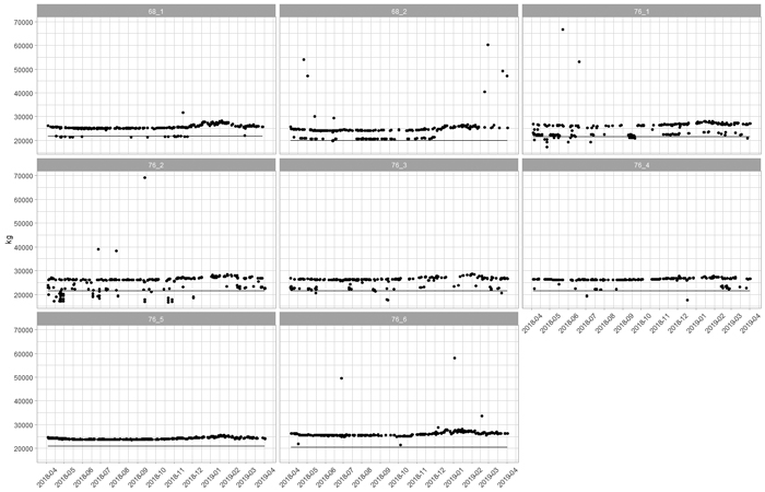
Fig. 1. Tare weight measurements of eight timber trucks over a year. The horizontal lines represent the tare weights in the national transport register (excluding the weight of a loader and other accessories). View larger in new window/tab.
2.2 Weather data
The Finnish Meteorological Institute provides data on certain weather variables in a grid format at 1 km × 1 km resolution (Finnish Meteorological Institute 2019). Such data at three-hour temporal resolution were retrieved for all the mill locations at the time of each delivery. The dataset included the following variables (resolution and unit in parentheses):
- temp = momentary temperature (0.1 °C)
- wind_speed = momentary wind speed (0.1 m s–1)
- rel_humid = momentary humidity (1%)
- prec = 3h rainfall (0.1 mm)
- pot_evap = 3h potential evaporation (0.1 mm).
2.3 Methods
The tare weight data included measurements that were not of interest from the annual variation point of view. First, in some cases a truck had only partially been unloaded showing very high tare weights (Fig. 1). This is why observations over 30 000 kg were removed. Second, due to fuel in the tank and equipment installed afterwards, the observed tare weight should always be higher than the registered one. Thus, values below the registered tare were deemed erroneous and removed.
Third, while most of the trips were driven with a loader attached, some of the trips were not. This can be seen as an additional layer below the tare weights with loader (Fig. 1). There was no information on the existence of a loader on a particular trip, so k-means classification (Hartigan and Wong 1979) was applied to separate the data into two clusters: with and without loader. Thereafter, the observations classified as without loader were removed.
In order to quantify how much of potential payload capacity was lost because of adhering snow so-called normal tare weight was first determined. Here it was defined as the 95th percentile of the tare measurements between 1 June and 31 August. This definition takes inherent variation due to, e.g., fuel level into account. Subsequently, the positive differences between observed tare and the normal tare outside the summer months were assumed to be equivalent to potential loss of payload (payload_loss_p95). In case the difference was negative, loss of payload was set to zero.
The effect of weather conditions on payload loss was assessed with regression models. The data were randomly divided into training and test data sets which comprised 80% and 20% of the observations, respectively. As the payload loss in the summer months was by definition practically zero, the observations between June and August were ignored.
To quantify the effects of weather on potential payload loss, a hierarchic two-step model with two component models was built. A logistic regression model was used to model whether payload loss occurs or not (the cases where the payload loss was zero) (Eq. 1) and a gamma regression with a logarithm as link function for the amount of payload loss for the cases where payload loss was observed (Eq. 2).
Both models can be written as generalized linear models (GLM) (where Y is the dependent variable, xi are model predictors and β is vector of model coefficients βi). The logistic regression model has the form

where μ = E[Y] is expected probability of payload_loss_p95 = 0.
The gamma regression for the positive payload_loss_p95 has the form of Eq. (2) with using mean parameterization for gamma distribution.

Model selection was done by using Bayesian information criterion (BIC) (Schwarz 1978). BIC is a model selection criterion which uses a penalty term for the number of parameters in a model to prefer simpler models and to reduce the possibility of overfitting. Likelihood-ratio test was used to assess model fit. The test compares goodness of fit of two statistical models based on the ratio of their likelihoods (Johnston and DiNardo 1997). The performance of the logistic regression model (Eq. 1) was evaluated with prediction accuracy (i.e. the number of correct predictions / the total number of predictions) and by using the F1 test score (Eq. 3).

where TP = number of true positive cases, FP = number of false positive cases and FN = number of false negative cases. The performance of the gamma regression (Eq. 2) was evaluated with the Root Mean Square Error (RMSE). The analysis was conducted in R (R Core Team 2020).
3 Results
3.1 Loss of payload
The filtered tare weights of the eight timber trucks are presented in Fig. 2. There were altogether 2250 remaining weight observations which ranged from 23 360 kg to 28 780 kg. The pattern of increasing weight in wintertime is clearly discernible. The figure also indicates the normal tare weights between June and August ranging from 23 900 kg to 26 390 kg.
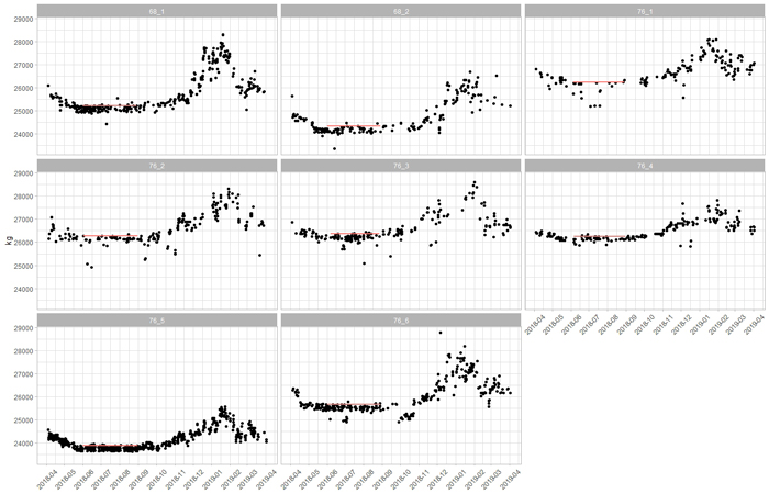
Fig. 2. Filtered tare weights of eight timber trucks over a year. The red lines indicate the normal tare, i.e., the 95th percentile of the tare measurements in summertime. View larger in new window/tab.
After subtracting the normal weights from the tare weights outside the summer months maximum loss of payload varied between 1560 kg and 3100 kg. On a monthly basis, the highest losses occurred in January, when the median values varied between 760 kg and 2180 kg (Fig. 3).
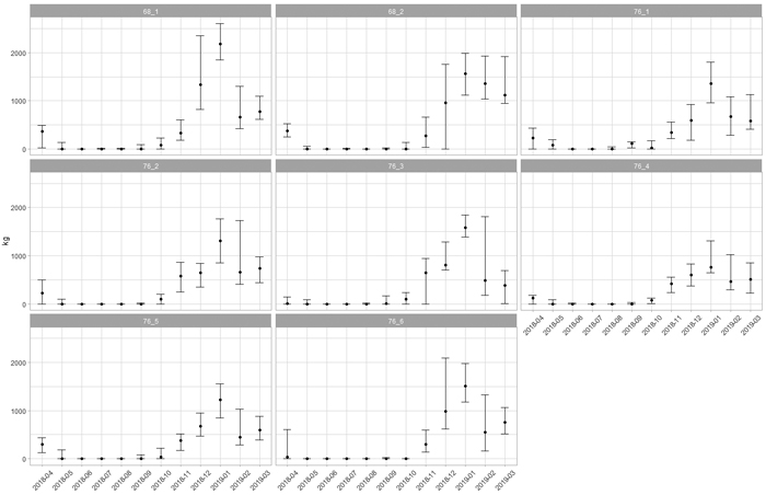
Fig. 3. Monthly median loss of payload of eight timber trucks over a year. The error bars indicate the 10th and 90th percentiles. View larger in new window/tab.
The equivalent loss of annual payload transported varied from 1.1 to 4.9 loads per truck representing from 0.5% to 1.5% of the total number of loads in the study (Table 2). However, in January the loss was equivalent to between 1.9% and 5.1% of the number of loads transported.
| Table 2. Equivalent annual loss of transport payload due to increased winter tare weight. | ||||||
| Truck id | Gross vehicle weight (kg) | Normal tare (kg) | Maximum payload (kg) | Annual loss of payload (kg) | Annual loss in payloads | Total loads per year in the study |
| 68_1 | 68 000 | 25 359 | 42 641 | 209 740 | 4.9 | 338 |
| 68_2 | 68 000 | 24 459 | 43 541 | 90 000 | 2.1 | 188 |
| 76_1 | 76 000 | 26 305 | 49 695 | 84 718 | 1.7 | 163 |
| 76_2 | 76 000 | 26 314 | 49 686 | 101 100 | 2.0 | 217 |
| 76_3 | 76 000 | 26 422 | 49 578 | 54 260 | 1.1 | 225 |
| 76_4 | 76 000 | 26 321 | 49 679 | 60 960 | 1.2 | 207 |
| 76_5 | 76 000 | 23 940 | 52 060 | 168 300 | 3.2 | 588 |
| 76_6 | 76 000 | 25 722 | 50 278 | 140 580 | 2.8 | 324 |
3.2 Effect of weather
The training data set consisted of 1800 observations. The highest correlations with payload loss were found for temperature, potential evaporation and relative humidity (Fig. 4). The correlation with rainfall was low, but highly significant.
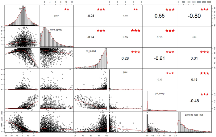
Fig. 4. Spearman correlation factors between payload loss and the weather variables in the training data. The variables (unit in parentheses): temp = momentary temperature (°C), wind_speed = momentary wind speed (m s–1), rel_humid = momentary humidity (%), prec = 3h rainfall (mm), pot_evap = 3h potential evaporation (mm), payload_loss_p95 = potential loss of payload (kg). Significance levels: *** = 0.001, ** = 0.01. View larger in new window/tab.
For modelling it was decided to investigate only three potential predictors: temperature, relative humidity and rainfall as well as their interaction terms. The best logistic regression predicting the probability for zero payload loss resulted in model coefficients in Table 3. The BIC value for the model was 887.353.
| Table 3. Model coefficients for logistic regression of probability of no payload loss. | ||||
| Term | Estimate | Standard error | z-score | p-value |
| Intercept | –2.29 | 0.125 | –18.3 | <0.001 |
| Temperature | 0.245 | 0.0153 | 16.1 | <0.001 |
The fitted model is significantly better than the null model in the likelihood-ratio test (Chi-squared test statistic = 527.005, df = 1, p-value < 0.001). The model’s prediction accuracy using a 50% cut-off point was 87.0% in the training data set and 87.5% in the test data set (Table 4). The F1 test score for the training data was 0.918 and for the test data 0.922 also indicating similar performance in both data sets. The confusion matrices of training and test data show similar behaviour in the both sets. The share of zero payload loss in training data was 23.1% and 20.8% in test data. Fig. 5 shows that the 50% probability for zero payload loss is roughly at 10 °C.
| Table 4. Confusion matrices for the prediction of zero / non-zero payload loss in the training and test data sets. | ||||
| Training data | Test data | |||
| Predicted non-zero payload loss | Predicted zero payload loss | Predicted non-zero payload loss | Predicted zero payload loss | |
| True non-zero payload loss | 949 | 48 | 231 | 16 |
| True zero payload loss | 121 | 178 | 23 | 42 |
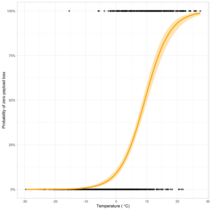
Fig. 5. Probability of zero payload loss as a function of temperature.
Of the tested regression models for payload loss (payload_loss_p95 > 0), the one including temperature, humidity, rainfall and their interaction terms as explanatory variables was the best compromise avoiding overfitting (Table 5). The BIC value for the model was 14478.010. The gamma family dispersion parameter (= 1/ν, i.e., the inverse of the shape parameter ν) was 0.403. The fitted model was significantly better than the null model in the likelihood-ratio test (Chi-squared test statistic = 378.653, df = 5, p-value < 0.001). The model performance measured by RMSE was 489 kg in the training data set and 439 kg in the test data set, which are of the order of a full fuel tank. The lower RMSE in the test data set can probably be explained by the lower variance in the test data than in the training data (standard deviation 571 kg and 603 kg, respectively). The model predictions as a function of temperature, humidity and rainfall are presented in Fig. 6.
| Table 5. Model coefficients of the gamma regression of positive payload loss. Notation a:b means an interaction term between variables a and b. | ||||
| Term | Estimate | Standard error | z-score | p-value |
| Intercept | 4.952 | 0.171 | 28.897 | <0.001 |
| Temperature | 0.033 | 0.020 | 1.635 | 0.102 |
| Relative humidity | 0.014 | 0.002 | 7.357 | <0.001 |
| Precipitation | 0.193 | 0.040 | 4.855 | <0.001 |
| Temperature: Relative humidity | –0.001 | 0.0002 | –5.513 | <0.001 |
| Temperature: Precipitation | –0.026 | 0.006 | –4.476 | <0.001 |
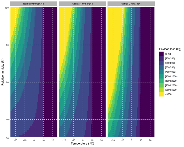
Fig. 6. The model for payload loss as a function of temperature, humidity and rainfall. View larger in new window/tab.
4 Discussion
The studied combination vehicles were typical in timber trucking in Finland. In 2018, the share of 76-, 68- and 60–64-tonners was 64%, 30% and 6%, respectively (Venäläinen and Poikela 2019). Although there were only eight trucks in the study, they represented a good variation in regard to geography and GVW. All of the trucks were of the same brand, but the trailers were from different manufacturers. According to the entrepreneurs, sometimes a lighter spare trailer had been used, which may explain some of the tare weights lower than the general level. With a bigger sample of trucks including different manufacturers the variation in payload loss would have been higher and even more extreme values probable.
The average temperatures in autumn (September–November) and winter (December–February) in 2018–2019 were not exceptional, but 1–2 degrees above the reference period 1981–2010 (Finnish Meteorological Institute 2020). Rainfall was close to the average of the reference period, except for autumn 2018, which was up to 40% drier than the average in some parts of the operating areas of the trucks. Higher rainfall might have increased payload losses depending on temperature.
The wintertime snow load on the trucks could have accumulated on any part of the route. Unfortunately, the routes were not known and the weather data were, therefore, only retrieved for the mill locations. Furthermore, unloading could have happened any time within the three-hour time window of the weather data. Consequently, in some cases the whole time of driving with a load has been included whereas only the delivery time in others.
The normal tare was defined as the 95th percentile of the tare measurements in summertime which excludes some extreme values but indicates the upper level of summertime tare weights. The selected approach omits negative outliers (i.e., the measured tare weight is clearly lower than the trend) which are lower than the normal tare but leaves all positive outliers. In theory, this could overestimate potential payload losses. However, there are not many such cases in the data (Fig. 2). In fact, the payload losses based on the 95th percentile can be considered conservative estimates as using summer averages would have yielded 120–310 kg higher payload losses.
All three entrepreneurs had chains in their trucks in winter. Trucks 68_1, 68_2, 76_5 and 76_6 were also equipped with sanding gear. Without knowing the exact dates when chains and sand were on board, their effect is very hard to estimate. All in all, the total weight of these could be hundreds of kilograms.
There were also considerable differences between the trucks’ normal weights. Of the two 68-tonners, truck 68_1 was almost one tonne heavier than truck 68_2. As a matter of fact, truck 68_1 was even 1.3 tonnes heavier than the lightest 76-tonne truck (76_5). The heaviest 76-tonner (truck 76_3) weighed around 2.4 tonnes more than the lightest one. A major reason for truck 76_5 being much lighter than the other trucks was that the loader was permanently fixed and it did not have a cabin. However, the optimal configuration of a combination vehicle also depends on the operating environment.
According to the results, payload loss starts to accumulate already when the temperature is above zero. This can at least partly be attributed to chains and sand, i.e., the entrepreneurs start to prepare for the winter conditions in advance. Payload loss further increased with decreasing temperature, and increasing humidity and rainfall (Fig. 4). Moreover, the higher was the relative humidity or rainfall the stronger was the effect of temperature (Fig. 6). For example, assuming no rainfall and 80% humidity a change of one degree at –10 °C implies approximately 65 kg change in payload loss. Correspondingly, a change of one degree at –10 °C at 90% humidity and 2 mm rainfall implies approximately 400 kg change in payload loss.
Payload loss has an influence on an entrepreneur’s profitability as potentially on average 1% more timber could have been transported. More importantly, there was a big difference between the best and the worst truck, which should act as motivation to pay attention to the reasons for high payload losses. Furthermore, January, February and March are the busiest months in timber transport and the highest payload losses occur just during the season of highest capacity utilization (Natural Resources Institute Finland 2020).
When considering the significance of payload loss at the national level, a rough calculation reveals the importance of the issue. In 2018, altogether 53.85 million m3 of domestic timber was transported in Finland with an average cost of EUR 7.05 m–3 (Strandström 2019). Assuming the average payload loss of 1% over a year, the loss equals 0.5 million m3 or EUR 3.6 million. Realizing that it is impossible to totally avoid payload losses, the theoretical losses at the national level should encourage the development of structures and materials of trucks and trailers. First, a more detailed study should be carried out to assess where exactly snow accumulates on different trucks and trailers.
With the present transport fleet it is essential to be able to load a truck so that the GVW (within the acceptable legal tolerance) is not exceeded. In summertime, loader scale measurement enables a driver to load a truck up to the GVW easier than in wintertime. In wintertime, the operators have to rely on their practical experience to estimate how much snow will accumulate during the trip. The model proposed in this study can also be used to support decision making on, e.g., when to pay attention on cleaning the truck to remove the accumulated snow and ice.
In conclusion, considerable increase of tare weights was observed with the studied trucks in wintertime. The study also showed that this loss of payload increased with decreasing temperature and increasing humidity and rainfall. However, further research is needed in order to test model’s performance in practice in different weather conditions and to create better models. The follow-up study should have a wider range of combination vehicles and accurate weather data from the whole trip of a truck. The results of the study also give incentive to develop truck and trailer structures that reduce the adherence of snow.
Acknowledgements
This work was financially supported by the Academy of Finland under the Climate-Neutral and Resource-Scarce Finland – Strategic Research Programme in 2015–2020 (Project FORBIO, No. 14970). The authors would like to thank forest companies Metsä Group, Stora Enso and UPM, and the three transport companies for providing the data for the study.
References
Asmoarp V., Enström J., Bergqvist M., von Hofsten H. (2018). Effektivare transporter på väg – slutrapport för projektet 2014–2018. [Improving transport efficiency – final report of the ETT 2014–2016 Project]. Skogforsk, Arbertsrapport nr. 962–2018. 65 p. [In Swedish].
Erlandsson E. (2008). Framgångsfaktorer för rundvirkesåkerier I Mellansverige. [Success factors for roundwood truck transport companies in mid-Sweden]. Sveriges lantbruksuniversitet, Arbetsrapport 230. 67 p. [In Swedish].
Finnish Meteorological Institute (2019). The Finnish Meteorological Institute’s open data. https://en.ilmatieteenlaitos.fi/open-data. [Cited 5 May 2020].
Finnish Meteorological Institute (2020). Temperature and precipitation maps from 1961 onwards. https://en.ilmatieteenlaitos.fi/maps-from-1961-onwards. [Cited 5 May 2020].
Hamsley A., Greene D., Siry J., Mendell B. (2007). Improving timber trucking performance by reducing variability of log truck weights. Southern Journal of Applied Forestry 31(1): 12–16. https://doi.org/10.1093/sjaf/31.1.12.
Hartigan J., Wong M. (1979). Algorithm AS 136: a k-means clustering algorithm. Journal of the Royal Statistical Society. Series C (Applied Statistics) 28(1): 100–108. https://doi.org/10.2307/2346830.
Heikkilä J., Lindblad J., Hujo S., Verkasalo E. (2004). Pienten kuitupuuerien mittaus puutavara-auton kuormainvaa’alla. [Measurement of small pulpwood lots with the loader scale of a timber truck]. Metsätieteen aikakauskirja 4: 527–540. https://doi.org/10.14214/ma.5669. [In Finnish].
Johnston J., DiNardo J. (1997). Econometric methods. Fourth edition. The McGraw-Hill Companies, Inc New York, NY.
Laitila J., Asikainen A., Ranta T. (2016). Cost analysis of transporting forest chips and forest industry by-products with large truck-trailers in Finland. Biomass and Bioenergy 90: 252–261. https://doi.org/10.1016/j.biombioe.2016.04.011.
Lehtonen I., Hoppula P., Pirinen P., Gregow H. (2014). Modelling crown snow loads in Finland: a comparison of two methods. Silva Fennica 48(3) article 1120. 30 p. https://doi.org/10.14214/sf.1120.
Malinen J., Nousiainen V., Palojärvi K., Palander T. (2014). Prospects and challenges of timber trucking in a changing operational environment in Finland. Croatian Journal of Forest Engineering 35: 91–100.
Marshall H., Murphy G. (2003). Factors affecting the accuracy of weighbridge systems. International Journal of Forest Engineering 14(1): 67–79. https://doi.org/10.1080/14942119.2003.10702471.
Natural Resources Institute Finland (2020). Industrial roundwood removals and labour force. https://stat.luke.fi/en/commercial-roundwood-removals-and-forestry-labour. [Cited 5 May 2020].
Palander T. (2016). Environmental benefits from improving transportation efficiency in wood procurement systems. Transportation Research Part D: Transport and Environment 44: 211–218. https://doi.org/10.1016/j.trd.2016.03.004.
Palander T. (2017). The environmental emission efficiency of larger and heavier vehicles – a case study of road transportation in Finnish forest industry. Journal of Cleaner Production 155(1): 57–62. https://doi.org/10.1016/j.jclepro.2016.09.095.
Peltola J. (2004). Puutavara-autojen rakenteen vaikutus omamassaan. [Effect of the structure of timber trucks on tare weight]. Metsätehon raportti 176. 23 p. [In Finnish].
R Core Team (2020). R: a language and environment for statistical computing. R Foundation for Statistical Computing, Vienna, Austria. https://www.R-project.org/.
Rönnqvist M. (2003). Optimization in forestry. Mathematical Programming 97: 267–284. https://doi.org/10.1007/s10107-003-0444-0.
Schwarz G. (1978). Estimating the dimensions of a model. The Annals of Statistics 6: 461–464. https://doi.org/10.1214/aos/1176344136.
Shaffer R., Stuart W. (2005). A checklist for efficient log trucking. Virginia cooperative extension Publication 420-094. Virginia Polytechnic Institute and State University. 5 p.
Strandström M. (2019). Puunkorjuu ja kaukokuljetus vuonna 2018. [Timber harvesting and transportation in 2018]. Metsätehon tuloskalvosarja 17a. 32 p. [In Finnish].
Trzciński G., Sieniawski W., Moskalik T. (2013). Effects of timber loads on gross vehicle weight. Folia Forestalia Polonica 55(4): 159–167. https://doi.org/10.2478/ffp-2013-0017.
Väätäinen K., Laitila J., Anttila P., Kilpeläinen A., Asikainen A. (2020). The influence of gross vehicle weight (GVW) and transport distance on timber trucking performance indicators – discrete event simulation study in case environment in Central Finland. International Journal of Forest Engineering 31(2): 156–170. https://doi.org/10.1080/14942119.2020.1757324.
Venäläinen P., Poikela A. (2019). Puutavara- ja hakeajoneuvojen massojen noston vaikutukset. [Effects of increased weights of timber and chip trucks]. Metsätehon raportti 253. 61 p. [In Finnish].
Total of 24 references.
Send to email

