Daesung Lee  ,
Jouni Siipilehto,
Jari Hynynen
,
Jouni Siipilehto,
Jari Hynynen
Models for diameter distribution and tree height in hybrid aspen plantations in southern Finland
Lee D., Siipilehto J., Hynynen J. (2021). Models for diameter distribution and tree height in hybrid aspen plantations in southern Finland. Silva Fennica vol. 55 no. 5 article id 10612. https://doi.org/10.14214/sf.10612
Highlights
- Parameter recovery method for the Weibull function fitted diameter distributions well by means of sum and mean forest stand characteristics for hybrid aspen plantations
- Arithmetic and weighted mean diameters performed better for the recovery method than the corresponding median diameters
- Two alternative Näslund’s height curve models with stand characteristics and tree dbh predictors provided unbiased tree height predictions.
Abstract
Hybrid aspen (Populus tremula L. × P. tremuloides Michx.) is known with outstanding growth rate and some favourable wood characteristics, but models for stand management have not yet been prepared in northern Europe. This study introduces methods and models to predict tree dimensions, diameter at breast height (dbh) and tree height for a hybrid aspen plantation using data from repeatedly measured permanent sample plots established in clonal plantations in southern Finland. Dbh distributions using parameter recovery method for the Weibull function was used with Näslund’s height curve to model tree heights. According to the goodness-of-fit statistics of Kolmogorov-Smirnov and the Error Index, the arithmetic mean diameter (D) and basal area-weighted mean diameter (DG) provided more stable parameter recovery for the Weibull distribution than the median diameter (DM) and basal area-weighted median diameter (DGM), while DG showed the best overall fit. Thus, Näslund’s height curve was modelled using DG with Lorey’s height (HG), age, basal area (BA), and tree dbh (Model 1). Also, Model 2 was tested using all predictors of Model 1 with the number of trees per ha (TPH). All predictors were shown to be significant in both Models, showing slightly different behaviour. Model 1 was sensitive to the mean characteristics, DG and HG, while Model 2 was sensitive to stand density, including both BA and TPH as predictors. Model 1 was considered more reasonable to apply based on our results. Consequently, the parameter recovery method using DG and Näslund’s models were applicable for predicting tree diameter and height.
Keywords
Näslund’s height curve;
Weibull distribution;
parameter recovery;
Populus tremula × P. tremuloides;
clonal plantation;
nonlinear mixed-effects model
-
Lee,
Natural Resources Institute Finland (Luke), Natural resources, Latokartanonkaari 9, FI-00790 Helsinki, Finland
 https://orcid.org/0000-0003-1586-9385
E-mail
daesung.lee@luke.fi
https://orcid.org/0000-0003-1586-9385
E-mail
daesung.lee@luke.fi
- Siipilehto, Natural Resources Institute Finland (Luke), Natural resources, Latokartanonkaari 9, FI-00790 Helsinki, Finland E-mail jouni.siipilehto@luke.fi
-
Hynynen,
Natural Resources Institute Finland (Luke), Natural resources, Vipusenkuja 5, FI-57200 Savonlinna, Finland
https://orcid.org/0000-0002-9132-8612
E-mail
jari.hynynen@luke.fi
Received 29 September 2021 Accepted 3 December 2021 Published 15 December 2021
Views 72816
Available at https://doi.org/10.14214/sf.10612 | Download PDF

Supplementary Files
1 Introduction
Hybrid aspen, a hybrid between the European aspen and North American trembling aspen (Populus tremula L. × P. tremuloides Michx.), is highlighted with great potential in modern wood production and biofuel forestry in northern Europe (Tullus et al. 2012; Fahlvik et al. 2019). Although it was first introduced for the matchwood industry in 1950s, as of today, plywood and veneer are one of the principal consumer goods because of the fibre characteristics and outstanding growth rate (Beuker 2000; Heräjärvi and Junkkonen 2006). Moreover, given the urgent need to mitigate climate change, hybrid aspen may play a significant role. First, due to its high growth rate, hybrid aspen plantation can uptake atmospheric carbon more rapidly than other northern tree species. Second, its use as bioenergy is expected to be accelerated in accordance with international conventions such as the Paris Agreement (Commission of European Communities 2008; European Commission 2013; United Nations Framework Convention on Climate Change 2015; Hytönen 2018).
Significant advantages of hybrid aspen in terms of growth characteristics and productivity based on clonal plantations have been reported in many studies (Hynynen et al. 2004; Luoranen et al. 2006; Stener and Westin 2017; Hytönen et al. 2018; Niemczyk et al. 2019). They generally concluded that hybrid aspen was a promising broadleaved species particularly for the region of coniferous-dominated forests such as those of northern Europe (Tullus et al. 2012; Fahlvik et al. 2019). The high growth and yield potential of hybrid aspen plantations has been observed in long-term experiments in Finland (Hynynen et al. 2002) and Sweden (Fahlvik et al. 2019). Nevertheless, growth and yield models for hybrid aspen have yet to be developed for stand management purposes (Stener et al. 2019). There is still a lack of modelling research except for a few studies carrying out the dominant height and site index model (Johansson 2013; Lee et al. 2021), thus highlighting the importance and necessity of developing stand- and tree-level models.
The choice of modelling approach depends on the characteristics of the stands to be modelled and their intended use. If stand structure is heterogeneous, e.g. including diverse tree species with a large variation of within-stand age or size, tree-level models instead of stand-level models are often preferred to better predict stand structure and dynamics (Somers and Nepal 1994; Quin and Cao 2006). However, in stands with a more homogeneous structure, such as even-aged, single-species plantations of clonal origin, the stand-level modelling approach is a viable option (Pienaar and Rheney 1995; Scolforo et al. 2019).
In practical forestry, forest inventory data often contain mean and sum values of measured stand characteristics, but seldom include information about individual trees. There are some differences of the collected stand characteristics between inventory methods. In the field inventory the mean characteristics are typically basal area-median dbh (DGM) and the corresponding height (HGM) due to the convenience to assess from the measured relascope sample plots. Such examples are the compartment-wise field inventory (CWFI) and the national forest inventory (NFI) (Koivuniemi and Korhonen 2006). In addition, the assessed stand characteristics for the advanced stands include basal area (BA) but do not include trees per hectare (TPH) in CWFI, NFI or in the open access Metsaan.fi service for stand compartments. Today, the area-based approach (ABA) for the airborne laser scanning (ALS) data for the 16 m × 16 m grid cells includes both BA and TPH together with basal area-weighted mean dbh (DG) and the Lorey’s height (HG) for Scots pine (Pinus sylvestris L.), Norway spruce (Picea abies (L.) Karst.) and broadleaves (Siipilehto et al. 2016). Thus, stand-level models are directly compatible with these data containing stand characteristics because stand-level models can be used to predict both stand dynamics (regeneration, growth, and mortality) and within-stand structure (diameter and height distributions). Information on trees’ within-stand size variation is necessary to assess timber assortments and the monetary value of the growing stock (Vanclay 1994). Further, size distribution models generate tree lists representing the stands, which are often used as input data of stand simulators applying individual-tree growth and yield models such as Motti in Finland (Salminen et al. 2005).
To generate a tree list that represents a stand, we need the diameter distribution of tree diameters at breast height (dbh), and a tree height model to complete the description for tree dimensions. Parameter prediction methods (PPM) for different distribution functions are already available, but none for hybrid aspen in Finland. There are several PPM in Finland, e.g. for the Weibull function (Kilkki and Päivinen 1986; Kilkki et al. 1986; Hökkä et al. 1991; Maltamo et al. 1995; Maltamo 1997; Siipilehto 1999, 2011) for predicting diameter distributions, mainly for Scots pine and Norway spruce but also for broadleaves (Siipilehto 1999). In addition, PPM for the more flexible Johnson’s SB distribution exists for pine, spruce, and birch in Finland (Siipilehto 1999; Siipilehto et al. 2013). Similarly, several height models have been presented in Finland (Lappi 1997; Mehtätalo 2004, 2005; Siipilehto 1999; Siipilehto and Kangas 2015), but none for hybrid aspen. Mehtätalo et al. (2015) showed the good performance of Näslund’s height curve among a large number of alternative height models and tree species. Further, Siipilehto and Kangas (2015) presented alternative Näslunds’s height curve models for Scots pine, Norway spruce, and birch species (Betula pendula Roth and B. pubescens Ehrh.) in Finland.
Siipilehto and Mehtätalo (2013) showed a superior result using the parameter recovery method (PRM) for 2-parameter Weibull distribution instead of PPM for Scots pine stands. However, only arithmetic mean dbh (D) and DGM were included when PPM and PRM were compared in terms of accuracy in volume characteristics (Siipilehto and Mehtätalo 2013). D and DGM obtained quite comparable accuracy, but D was slightly better for young stands, whereas DGM performed slightly better for advanced stands in terms of bias and RMSE in volume characteristics (Siipilehto and Mehtätalo 2013). Thus far, we have no evidence about how the median dbh (DM) or DG perform with the parameter recovery method. No matter which mean or median dbh is selected, the recovered distributions can provide it correctly with TPH and BA. The alternative mean or median can therefore be assumed to provide quite comparable results.
The general objective of this study was to develop methods and models for predicting individual tree dimensions (dbh and height) in hybrid aspen plantations. The specific objectives were: i) to test the optional mean and median characteristics for the PRM in solving diameter distribution; and ii) to develop the tree height models with the best performing stand characteristic. Diameter distribution with the height-diameter relationship provided the final models and methods for predicting tree dbh and height for hybrid aspen.
2 Materials and methods
2.1 Modelling data
Data for modelling were collected in clonal hybrid aspen plantations in southern Finland, which had been designed for assessing the effects of varying initial planting densities in four different locations (i.e. experiments). The experiments were established in Lohja, Jalassaari (60°13´N, 23°56´E), Lohja, Kirkniemi (60°11´N, 23°57´E), Lapinjärvi (60°39´N, 26°08´E), and Pornainen (60°32´N, 25°20´E) in Finland, and comprised of 4–24 plots with a plot area of 1000 m2 by location (Lee et al. 2021). The experiments were repeatedly remeasured 7–12 times by site between 1997 and 2016. The detailed information on clones, plot design, and the history of silvicultural treatment was described in Lee et al. (2021). In each plot, dbh and height were measured for all trees.
A variety of stand- and tree-level characteristics such as stand age (AGE), stand density in terms of TPH and BA, diameter, and height were used for modelling tree dimensions (Table 1). Among them, four kinds of mean or median dbh were analysed to find the best option for the parameter recovery method: D, DG, DM, and DGM with quadratic mean dbh (DQ) squared as a second moment (Table 1). Dominant height (HDOM) was calculated by averaging tree height of one hundred trees with the largest dbh per ha. Site index (SI) was computed based on the density-sensitive site index model suggested by Lee et al. (2021).
| Table 1. Summary statistics of modelling data to test parameter recovery method of Weibull distribution and to develop Näslund’s height curve model for hybrid aspen (Populus tremula × P. tremuloides) from southern Finland. | |
| Variables | Statistics, Mean ± SD (Min–Max) |
| Dataset structure | |
| No. of stands | 4 |
| No. of plots | 48 |
| No. of sample trees | 4481 |
| No. of measurements by stand | 7–12 |
| No. of observations at plot-level instances | 294 |
| No. of observations at tree-level instances | 26 933 |
| Stand characteristics | |
| Stand age (AGE, years) | 5–20 |
| Stand density (TPH, trees ha−1) | 930 ± 423 (300–1600) |
| Basal area (BA, m2 ha−1) | 10.8 ± 9.0 (0.1–35.7) |
| Diameter, arithmetic mean (D, cm) | 11.1 ± 5.6 (1.5–24.9) |
| Diameter, basal area-weighted mean (DG, cm) | 12.0 ± 5.7 (2.1–26.8) |
| Diameter, median (DM, cm) | 11.3 ± 5.8 (1.2–26.0) |
| Diameter, basal area median (DGM, cm) | 12.1 ± 5.8 (1.9–26.6) |
| Diameter, quadratic mean (DQ, cm) | 11.4 ± 5.6 (1.8–25.4) |
| Height, basal area-weighted mean (HG, m) | 13.5 ± 6.6 (3.6–27.6) |
| Dominant height (HDOM, m) | 15.1 ± 6.7 (4.0–29.8) |
| Site index a (SI, m) | 25.5 ± 2.7 (17.5–29.9) |
| Tree characteristics | |
| Diameter at breast height (dbh, cm) | 10.8 ± 5.7 (0.1–31.8) |
| Height (h, m) | 13.6 ± 6.8 (1.4–31.4) |
| a: Site index was computed based on Lee et al. (2021) with a base age of 20 years. | |
2.2 Models for tree dimensions
2.2.1 Parameter recovery method for dbh distribution
We applied the 2-parameter Weibull function to characterize dbh distributions. The 2-parameter Weibull probability density function (f) is as follows:
![]()
where x is the random variable, the observed diameter of a tree in a plot, and b and c are the scale and shape parameters of the Weibull function respectively. The computation of quantiles (e.g. median) is easy due to the closed-form cumulative Weibull function:
![]()
Parameter recovery equations for the 2-parameter Weibull distribution are presented in Siipilehto and Mehtätalo (2013) for the optional mean and median characteristics: D, DG, DM, and DGM. The corresponding recovery equations are as follows:
![]()

![]()

With the mean or median characteristics, we need the second raw moment for the recovery. The second moment of diameter distribution is as follows:
![]()
In the previous equations, the gamma function ![]() is a shortcut for the integral,
is a shortcut for the integral,  F–1(y) is the quantile function of Y that is the inverse function of the standard Gamma cumulative density function, and DQ is the quadratic mean dbh (Siipilehto and Mehtätalo 2013).
TPH and BA are used to define the second moment, which is DQ2 = BA/(TPH × q), in which q is a conversion factor π/2002 = 7.854E−05. Note that the square root of the second raw moment is the quadratic mean diameter (DQ). We applied the recovery equations by Siipilehto and Mehtätalo (2013), utilising their supplementary file Weibull2recovery.r for solving the two parameters of the Weibull function (also found as recweib function in lmfor package by Mehtätalo and Kansanen (2020)). The Newton-Raphson method for root finding was used to resolve the parameters of the system of two non-linear equations.
2.2.2 Prediction for individual tree height
We used the Näslund height curve (Näslund 1936) model as a base function to predict individual tree height (h). Näslund’s function is as follows:
![]()
where b0 and b1are the estimated parameters. Power 2 in Eq. 8 was selected for hybrid aspen as a light demanding species. Note that power 3 has been used for shade-tolerant species, e.g. Norway spruce and European beech (Fagus sylvatica L.), for flexibility to the sigmoid curve (Vestjordet 1972; Siipilehto 1999; Nord-Larsen 2006; Siipilehto and Kangas 2015). We used the lmfor package (Mehtätalo 2015) of the R statistical software (R Core Team 2019) and the exponential formulation for Näslund’s height curve HDNaslund4, in which tree height is as follows:
![]()
One of the benefits in this formulation is that b0 and b1 are always given a positive value that is needed for logical behaviour. In addition, Siipilehto (2011) showed the linear relationship between the logarithmic parameter ln(b1) and logarithmic Lorey’s height ln(HG), as well as the logarithmic dominant height ln(HDOM).
In b0 and b1 parts of Eq. 9, we attempted to add several stand-level characteristics as predictors, e.g. DG, HG, AGE, BA, TPH, and SI. Several transformations such as square root, logarithm, and reciprocal form and intercepts (k) ranging from 0.1 to 5.0 were also checked to identify the most stable and unbiased model performance, e.g. ln(BA + k), 1/(AGE + k) (see Siipilehto 2011; Siipilehto and Kangas 2015).
2.3 Statistical approach and model validation
2.3.1 Validation of dbh distributions
We evaluated the goodness-of-fit of the Weibull distribution, which was solved by the optional mean and median dbh characteristics for the parameter recovery (Eqs. 3–6). The goodness-of-fit tests included the Kolmogorov-Smirnov (KS) test, using an alpha (α) 0.1 risk level. When the number of sampled trees (n) exceeded 100, the approximate critical value was calculated according to Sokal and Rolf (1981) as √(ln(α/2)/2n). When the calculated test value (supremum) was related to critical value as a KS quotient (KSq), the quotient value above 1 indicated rejection (Tham 1988; Siipilehto et al. 2016). The number of rejected cases was counted for each optional recovery equations. In addition, the Error Index (EI) of Reynolds et al. (1988) was used for evaluation. EI is the sum (or weighted sum) of the absolute errors in the real frequencies by dbh class. In this study, the differences were calculated in 1-cm dbh classes without weighting. The smaller the test value of KS and EI, the better the fit.
In addition to the assessment of KS test and EI, the recovered dbh distributions were checked by illustrating with the observed dbh distribution. Based on the comparison between the observed and predicted number of trees by dbh class, the best model prediction was verified as stable and reasonable with every stand, plot, and age measurement instances of our dataset.
2.3.2 Modelling height curve
A nonlinear mixed-effects regression for Eq. 9 was applied for the Näslund’s height curve. We used experiment (four locations) as random effects for both intercept (b0) and coefficient (b1). Logarithmic transformations of stand characteristics showed the best performance for the Näslund’s height curve. The final mixed-effects model can thus be written as follows:
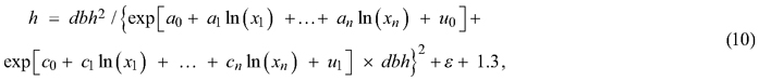
where a0 – an are estimated parameters for the intercept and predictor variables ln(x1) – ln(xn) for the Näslund’s parameter b0 in Eq. 9, c0 – cn are the estimated parameters for the intercept and the predictor variables ln(x1) – ln(xn) for the Näslund’s parameter b1 in Eq. 9, u0 is the random intercept and u1 is the random coefficient representing the four experiments, and ε is the residual error. For model development, we used the nlme package of the R statistical software (R Core Team 2019), and the initial values and the initial model structure for parameter fitting were referenced from the preceding study (Siipilehto and Kangas 2015). The power function was used to take into account the heteroscedasticity of the residual error ε with respect to predicted tree height, i.e. weights = varPower().
The modelling results were basically evaluated with the basic fit statistics: AIC, BIC, and –2Log likelihood. For the candidate models, residual plots of the dependent variable over each independent variable were carefully examined to assure the unbiased model fit by using the fixed-effect parameters without estimated random effects. Moreover, residuals against the social status of a tree (dbh/DG) were examined (Siipilehto 2011; Siipilehto and Kangas 2015).
The height models were demonstrated by applying only fixed-effects parameters with measured height-dbh scatterplots. Finally, the most representative and illustrative examples were presented to obtain information about model behaviours with respect to dbh distributions and height-dbh relationship, also without random effects.
3 Results
3.1 Comparison of the parameter recovery equations
In all the cases the converged solution was found. The goodness-of-fit results clearly showed superior performance for mean characteristics (D and DG) than the median characteristics (DM and DGM) (Table 2). DM (Eq. 5) provided the worst results, and the average KSq greater than 1 implied that the recovered distributions frequently rejected the KS test at the α 0.1 level. The number of rejected cases at the α 0.1 level was 101 (34%) out of 294 total cases using DM. In contrast, DG (Eq. 4) provided the best goodness-of-fit results, and only 8 cases (2.7%) rejected the KS test at the α 0.1 level (Table 2). The first moment, D (Eq. 3) provided the second-best result with 5.1% rejected cases, while the result of DGM (Eq. 6) was 12.6% (Table 2). Most of the rejected cases using DG occurred in young stands where the dbh distribution was still narrow and the predicted mode class was typically 1 cm higher than the observed mode class, e.g. the observed mode class was 4 cm and the predicted mode class was 5 cm.
| Table 2. The goodness-of-fit statistics for the recovered Weibull functions using arithmetic mean (D), basal area weighted mean (DG), median (DM), and basal area median dbh (DGM) for resolving the parameters based on the data of hybrid aspen (Populus tremula × P. tremuloides) from southern Finland. The smaller the value of test criterion, the better the fit. The values are mean ± standard deviation with minimum-maximum in parentheses. | ||||
| Variable | Kolmogorov-Smirnov quotient | Rejection cases of Kolmogorov-Smirnov at 10% level | The proportion of rejected cases to 294 total cases (%) | Error index by Reynolds et al. (1988) |
| D | 0.535 ± 0.232 (0.054–1.478) | 15 | 5.1 | 23.29 ± 11.52 (0.67–56.43) |
| DG | 0.507 ± 0.213 (0.134–1.425) | 8 | 2.7 | 22.75 ± 11.19 (2.67–60.31) |
| DM | 1.463 ± 2.673 (0.175–29.528) | 101 | 34.4 | 50.73 ± 58.38 (4.83–470.71) |
| DGM | 0.675 ± 0.741 (0.064–11.212) | 37 | 12.6 | 26.41 ± 13.11 (1.39–91.62) |
| Note: Kolmogorov-Smirnov quotient is the supremum divided by the critical value. | ||||
The box and whisker plots presented the distribution of calculated KSq (a) and EI (b) statistics by four age classes (Fig. 1). According to these results, D showed a slightly better fit for the youngest state of the stand than DG. In the oldest state (age ≥18 years) DG and DGM showed equal and best KSq, but simultaneously, DG had slightly smaller EI (Fig. 1). Overall, the central location of statistics was lowest in an order of DG < D < DGM < DM. DM especially presented a lengthy quartile range, skewed pattern, and large mean value due to extreme outliers, which implies an unstable estimation. In an early age class, the median of KSq statistic was 0.47 for D and 0.50 for DG (Fig. 1a). However, using DG for recovery provided the most constant results across all the age classes. The KS and EI goodness-of-fit results encouraged us to select DG as a candidate predictor variable for modelling the height-dbh relationship.
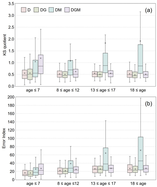
Fig. 1. Box and whisker plots of Kolmogorov-Smirnov quotient (KSq, plot a) statistics and Error Index (EI, plot b) by parameter recovery method of Weibull function for diameter distribution of hybrid aspen (Populus tremula × P. tremuloides) in southern Finland. The colour legend indicates different diameter types: D is the arithmetic mean diameter (cm); DG is the basal area-weighted mean diameter (cm); DM is the median diameter (cm); DGM is the basal area median diameter (cm). Each symbolic shape indicates the specific statistic as follows: the centre horizontal solid line inside the box is the median; the × mark is the mean; the lower boundary of the box is the 1st quartile (Q1); the upper boundary of the box is the 3rd quartile (Q3); the vertical length of the box is the interquartile range (IQR, Q3–Q1); the minimum value within the lower whisker below the box is the smallest observation above Q1–1.5×IQR; and the maximum value within the upper whisker above the box is the largest observation below Q3+1.5×IQR.
To illustrate the parameter recovery method of the Weibull function, three representative cases of probability distribution presented fitting accuracy. These plots were deliberately chosen by each stand condition to show how different solutions could be provided based on the four kinds of recovery equation, and the results were thus distinctively presented in Fig. 2. In most cases of the studied plots, the recovered Weibull distributions fitted the observed dbh distributions well. In the relevant example in this case, for D, DG, DM, and DGM, KSq was 0.518, 0.485, 0.573, and 0.616, and EI was 30.4, 29.5, 37.7, and 34.1 respectively (Fig. 2a). In some other cases, there was a greater difference between the parameter recovery equations. For example, in the case of Fig. 2b, the shape of the distribution using DGM was too peaked (rejected KS test), whereas DM resulted in too flat a distribution (but it still passed the KS test).
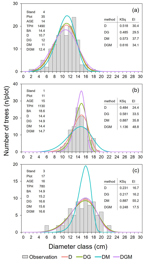
Fig. 2. Examples of the recovered Weibull distributions for three plots with fit statistics in clonal hybrid aspen (Populus tremula × P. tremuloides) plantations in southern Finland. The stand characteristics of each case are presented together on the left of the subplot. The fit statistics corresponding to each case are provided on the right with KSq and EI to compare the diameter types for the recovery method of Weibull distribution. KSq is the Kolmogorov-Smirnov quotient (supremum/critical value). EI is the Error Index (Reynolds et al. 1988). All the other abbreviations indicate stand characteristics as follows: AGE is the stand age (year); TPH is the number of trees per ha (trees ha−1); BA is the stand basal area (m2 ha−1); D is the arithmetic mean diameter (cm); DG is the basal area-weighted mean diameter (cm); DM is the median diameter (cm); DGM is the basal area median diameter (cm).
Moreover, in extreme cases, the recovered distributions using DM evidently deviated from the observed distribution, resulting in large KSq and EI of the DM (Eq. 5) option (Table 2, Fig. 1). A representative plot of this type was shown in plot 17 of stand (i.e., experiment) 3 at age 16 (Fig. 2c), although the KSq of every method still passed the KS test in this case (KSq < 1.0). Unlike the other parameter recovery options, DM resulted in a poor fit with the observed distribution. Specifically, the KSq value of 0.887 and the EI of 55.2 using DM were much higher than with the other options: KSq 0.217–0.248 and EI 16.2–17.5 for D, DG, and DGM. In some cases, the highest KSq values (KSq > 3) were caused by distributions where almost all the predicted trees’ dbh was about the same as DM. Overall, the goodness of fit varied depending on the stand condition as presented in the examples. Nonetheless, the performances when using D and DG for recovery were the most stable, while several unstable cases used DM and DGM.
3.2 Models for individual tree height
The formulation of Näslund’s height model included various stand characteristics such as age, stand density, mean diameter, and mean height. Model fitting with logarithmic transformation performed well. Finally, the chosen predictors were the logarithm of DG, HG, AGE, BA, and TPH. SI was not significant due to the correlation with DG, HG, and AGE, so it was excluded. The finally proposed two model formulas for fixed effects are respectively as follows:
in Model 1
![]()
![]()
and in Model 2
![]()
![]()
where b0 and b1 of Model 1 and Model 2 are the parameters for Näslund’s exponential Eq. 9, a0 – a5 are the estimated parameters of each equation in this study, and the other terms are as previously defined.
The fit statistics of the final models were the best among the tested models, and all the fixed-effect parameters were highly significant (P < 0.0001) (Table 3). The standard deviation of random effects was similar, and the power for weighting was larger in Model 1 (Table 3). Because the random effects were significant for intercept (b0) and coefficient (b1), both the shape and the asymptote of the height curve changed between the four experiments. Overall, the fit statistics of the AIC, BIC, and −2Log-likelihood were better in Model 2, which was the result of adding the predictor of stand density, TPH. Compared with the absolute values of predictors, DG and HG were larger in Model 1 than in Model 2. The opposite sign in the parameter for ln(DG) and ln(HG) also resulted in Model 1 following the changes in these mean characteristics. In Model 2, the parameters of DG and HG were relatively low, whereas those of BA and TPH were larger in Model 2, which reflects the higher impact caused by stand density.
| Table 3. Parameter estimates and fit statistics for Näslund’s height curve models to predict individual tree height of hybrid aspen (Populus tremula × P. tremuloides) in southern Finland. | |||||||
| Model 1 | Model 2 | ||||||
| Estimate | S.E. | Estimate | S.E. | ||||
| Fixed effects | b0 | a0 | Intercept | −0.2531 | 0.0493 | 0.4180 | 0.0592 |
| a1 | ln(DG) | 0.4124 | 0.0229 | 0.3788 | 0.0204 | ||
| a2 | ln(HG) | −0.2723 | 0.0285 | −0.2585 | 0.0254 | ||
| a3 | ln(AGE) | −0.1683 | 0.0263 | −0.2184 | 0.0227 | ||
| a4 | ln(TPH) | −0.0658 | 0.0060 | ||||
| b1 | a0 | Intercept | −0.4411 | 0.0093 | 2.3409 | 0.0420 | |
| a1 | ln(DG) | 0.1277 | 0.0069 | −0.4653 | 0.0107 | ||
| a2 | ln(HG) | −0.4804 | 0.0100 | −0.5922 | 0.0093 | ||
| a3 | ln(AGE) | −0.0431 | 0.0082 | 0.0479 | 0.0071 | ||
| a4 | ln(BA) | −0.0156 | 0.0012 | 0.3039 | 0.0044 | ||
| a5 | ln(TPH) | −0.2880 | 0.0043 | ||||
| Random effects | u0 | std(experiment) | 0.0851 | 0.0663 | |||
| u1 | std(experiment) | 0.0097 | 0.0190 | ||||
| Corr(u0, u1) | –0.413 | –0.998 | |||||
| Residual | std(ε) | 0.2489 | 0.2719 | ||||
| Variance function | Power | 0.4459 | 0.3769 | ||||
| Fit statistics | AIC | 60 500.64 | 56 125.17 | ||||
| BIC | 60 615.46 | 56 256.38 | |||||
| –2logLik | 60 472.64 | 56 093.16 | |||||
| AIC is the Akaike information criterion. BIC is the Bayesian information criterion. –2logLik is the –2 × log-likelihood value. Corr is the correlation between random-effect parameters. All the fixed-effect parameters were highly significant (P < 0.0001). | |||||||
In residual plots, all the predictors used in models, including DG, HG, AGE, BA, TPH, and tree dbh, were unbiased, showing a random distribution of residuals (Supplement file S1). To validate the models with a tree’s social status, an additional residual plot was analysed over dbh divided by DG, which represents the relative dominance in a stand. A subtle bias of the residuals over dbh/DG was detected in the middle range of Model 1 (Fig. 3a). On the other hand, the residuals were completely unbiased throughout the whole range of dbh/DG with Model 2 (Fig. 3b). Simultaneously, the residual errors were clearly diminished in Model 2 (Fig. 3b) compared with Model 1 (Fig. 3a).
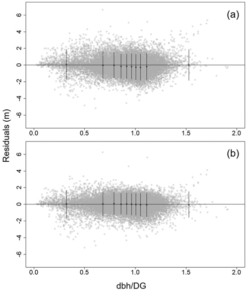
Fig. 3. Residual plots of Näslund’s Model 1 (a) and Model 2 (b) against the social status of a tree, dbh/DG to predict tree height of hybrid aspen (Populus tremula × P. tremuloides) in southern Finland. The selected variables and formulas are provided in Eqs. 11 and 12 for Model 1 (a), and Eqs. 13 and 14 for Model 2 (b). Note that here the residual analysis was performed only with fixed-effect parameters for general purposes. The whiskers were offered by the lmfor package in R statistical software to detect any bias (Mehtätalo 2015).
To test the goodness of fit in individual tree height estimation, two examples of Näslund’s model application were displayed in Fig. 4. As the scatterplot of stand (experiment) 1, plot 26, age 11, there were many cases where the predicted value of Model 1 was a little higher than Model 2 (e.g. Fig. 4a). On the other hand, the scatterplot of height-dbh allometry in stand 1, plot 32, age 18, the predicted height curve of Model 1 was a little lower than Model 2 (e.g. Fig. 4b). Other than these cases, no case showed a noticeable difference between models.
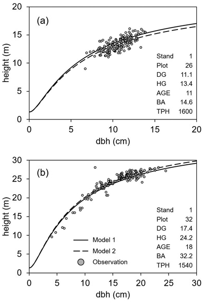
Fig. 4. Examples of the observed tree dimensions and the predicted height curves according to Näslund’s height models developed in this study for hybrid aspen (Populus tremula × P. tremuloides) in southern Finland. Note that the predictions are based on the fixed-effect parameters of Model 1 and Model 2 in Table 3. The stand characteristics of each case are shown together on the right of the plot and all the abbreviations are as follows: DG is the basal area-weighted mean diameter (cm); HG is the basal area-weighted mean height (m); AGE is the stand age (year); BA is the stand basal area (m2 ha−1); TPH is the number of trees per ha (trees ha−1).
However, in most of the studied sample plot cases, the height estimation difference was so subtle that both models were considered reasonable in reality. In addition, both models fitted well throughout all stand characteristics. One different feature was the sign of the estimated parameters for ln(DG) and ln(HG), and its impact on the model equation. Because of the opposite signs for these parameters, Model 1 was more closely driven by DG and HG. In contrast, DG and HG in Model 2 had a relatively minor impact on tree height prediction. This was because the estimated effects of DG and HG for the Näslund’s parameter b1 were both negative (effect of DG turned from positive in Model 1 to negative in Model 2). Instead, the impact of stand density was strong because of both predictor variables, BA and TPH, in Model 2.
4 Discussion
4.1 Performance of diameter distribution model
Hyink and Moser (1983) showed the basics when it comes to recovery methods in general. Traditionally, the first moment (D) has been used for the parameter recovery of the Weibull function (Burk and Newberry 1983). Cao (2004) used the traditional first moment (D) for parameter recovery and obtained reasonable results, e.g. the second-best KS test result when comparing alternative prediction methods in his study. Sometimes, the parameter recovery method has been a kind of hybrid utilising both moments and percentiles such as median (DM as 50th diameter percentile) (Baldwin and Feduccia 1987; Liu et al. 2009). Nevertheless, the differences in the recovery performance between the alternative mean and median characteristics were unknown.
In our study, DG (Eq. 4) provided the overall best KS goodness-of-fit results for the recovered dbh distributions. The proportion of rejected cases was far less (2.7%) than the risk level of 10% (Table 2). The main reason for rejection was 1-cm discrepancies in the dbh class between the predicted and observed mode, and this mostly happened in the early state of stands (6 out of 8 rejected cases belonged to the first measurement occasion). The first moment (D) provided a better result than DGM (Eq. 6), as in the paper by Siipilehto and Mehtätalo (2013) for young Scots pine stands. DGM has typically been a defined characteristic in forest management planning fieldwork as an easily defined median tree of the relascope sample plot. Today, when management planning is based on ALS data, DG has replaced DGM because of a straightforward calculation, i.e. ∑dbh3/∑dbh2 (Siipilehto et al. 2016).
DM (Eq. 5) clearly provided the most unstable fit results, and the proportion of rejected cases was as high as 34%. The estimated parameter c was sometimes so high (c > 20) that all the trees were practically of the same size when using DM. Note that the median is less sensitive than the mean for small changes in dbh. This means the sample mean is a statistically more efficient estimator than the median. Because of this feature, the recovery methods using mean characteristics in our study reflected the distributions of the observed tree dbh more similarly than those using median characteristics. Taking the stable solution and the lowest KS and EI across the whole range into account, DG is considered the best option for the parameter recovery of the Weibull function. Based on this finding, DG can hence be further used as a promising dependent variable to develop the stand-level model for the mean diameter of hybrid aspen plantation.
4.2 Performance of tree height model
Model 2 has better fit statistics than Model 1, but Model 1 was more sensitive to changes in the mean dimensions DG and HG, while Model 2 was more obviously affected by stand density such as BA and TPH. Among every candidate model examined in this research, Model 1 and Model 2 were finally chosen because fit statistics were the best, and the estimated parameters were all highly significant (P < 0.0001). The residuals over all predictors also showed unbiased patterns without an abnormal trend. Both models can thus be applied especially within the fitted data range when stand characteristics are considered.
When dbh/DG representing social status was also checked, a slight bias was detected in the middle of the dbh range for Model 1 (Fig. 3a). As reported in Siipilehto and Kangas (2015), the tree heights for trees of average size were slightly overestimated. Nonetheless, Model 1 is still considered a compelling formula, because the height-dbh relationship followed the mean dimensions, DG and HG, well. Meanwhile, Model 2 placed more weight on stand density, BA and TPH, but did not behave as logically with respect to DG and HG as Model 1. Model 1 would therefore be safer and more reasonable to estimate individual tree height especially for extrapolation ranging beyond our modelling dataset, e.g. TPH. In addition, the strong correlation between the random effects (–0.998) may indicate overparameterizing of the Model 2.
Model 2 including TPH presented slightly better fit statistics and residuals over dbh/DG, but Model 1 is still considered desirable and viable for general stand condition, e.g. predicting beyond the range of the modelling data. Overall, Näslund’s models for tree height prediction are assessed to implicitly include the feature of the site index with the density effect caused by the interaction among AGE, DG, HG, BA, and/or TPH. According to common knowledge, stand density affects competition among trees, and it thus affects stem taper. This feature was performed in both height models. SI depicts stand carrying capacity and yield. On more fertile sites, the trees are taller than on less fertile sites at a given age. However, this feature was more or less characterised through AGE, DG, and HG, especially in Model 1. Model 1 is therefore expected to offer a flexible and suitable prediction according to varying stand condition.
4.3 Applicability and practicability of the final models
The developed models were designed to be used in practice after taking the modelling data range into account. The number of trees per hectare in this study ranged from 400 to 1600, which are sparser than the prevailing practice in Finland (Hynynen et al. 2002; Lee et al. 2021). In addition to the compliance with these conditions, DG was evaluated as the most stable characteristic for recovering diameter distribution as presented in this study (Table 2, Fig. 1, Fig. 2).
When predicting tree height using Näslund’s model, extrapolation should be cautiously reviewed with the stand age applied in the field, because Models 1 and 2 in this study were developed with the predictor of AGE, ranging from 5 to 20 years. According to the current silvicultural guideline in southern Finland for broadleaved species such as silver birch, the mean diameter range of 27–32 cm is recommended for final felling (Rantala 2011). Based on the maximum mean diameter of our data, the age of 20 years is already close to suitable rotation age for hybrid aspen (Table 1). Furthermore, since the height and dominant height in this study differed significantly by initial stand density (Lee et al. 2021), it is distinguishing that Näslund’s model for hybrid aspen included the predictors of HG and BA which dynamically responded to the stand density effect (Table 3). Considering that Model 1 was sensitive to dimensions DG and HG while Model 2 was highly sensitive to stand density such as TPH and BA, Model 1 is evaluated as more practicable with parsimonious input variables than Model 2.
5 Conclusion
In this study, tree-level methods and models were studied for a clonal hybrid aspen plantation using empirical data collected from southern Finland. Four kinds of mean diameter were examined to identify the best-performing equation for the parameter recovery of the Weibull function. The comparison was successfully conducted with meaningful fitting differences. This was the first study to present evidence that the selected mean characteristic has a significant effect on the goodness-of-fit for the recovered dbh distributions. Both the arithmetic and weighted mean characteristic (D, DG) performed better than the corresponding median dbh (DM, DGM). DG generally provided the best fit results, and it was therefore selected as an input variable for height-curve modelling. Note that DG is included in the stand characteristics assessed from the current ALS data.
Näslund’s height curve showed excellent fit to data with fundamental stand- and tree-level variables, including AGE, DG, HG, and tree dbh. Variables describing stand density such as BA and TPH were also successfully added to the model, implying a significant stand density effect on tree height: only BA in Model 1 and both BA and TPH in Model 2. None of the models were biased against predictors according to residual plots. A slight bias in a tree’s social status (dbh/DG) using Model 1 was corrected in Model 2. However, despite the slightly worse fit statistics, Model 1 showed more logical behaviour in changes in mean characteristics as the tree height curves always followed the DG and HG. Thus, it was evaluated to be safer to apply Model 1 in a simulator.
Declaration of openness of research materials, data, and code
The study material and data were obtained from the Natural Resources Institute Finland (Luke), and it is confidential and unavailable without separate permission. The used code (R statistical software) is available from the Supplementary file S2.
Authors’ contributions
Daesung Lee: conceptualisation, methodology, formal analysis, software, visualisation, writing – original draft, writing – review and editing, funding acquisition.
Jouni Siipilehto: conceptualisation, methodology, writing – original draft, writing – review and editing, validation.
Jari Hynynen: data maintenance, methodology, writing – review and editing, validation, supervision, project administration, funding acquisition.
Declaration of Competing Interest
The authors declare no conflict of interest.
Acknowledgements
Research work was carried out in the Natural Resources Institute Finland (Luke), which also provided the empirical data for the analyses.
Funding
This research was supported by the ModSim project (Modelling and simulation of stand structure and development) funded by the Natural Resources Institute Finland (Luke) in 2021 and by the Basic Science Research Programme through the National Research Foundation of Korea (NRF) funded by the Korean Ministry of Education (Grant No. NRF-2019R1A6A3A03032912) in 2019.
References
Baldwin VC Jr., Feduccia DP (1987) Loblolly pine growth and yield prediction for managed West Gulf plantations. USDA Forest Service, Research Paper SO-236. https://doi.org/10.2737/SO-RP-236.
Beuker E (2000) Aspen breeding in Finland, new challenges. Balt For 6: 81–84.
Burk TJ, Newberry JD (1984) A simple algorithm for moment-based recovery of Weibull distribution parameters. For Sci 30: 329–332.
Cao QV, Burkhart HE (1984) A segmented approach for modeling diameter frequency data. For Sci 30: 129–137.
Commission of the European Communities (2008) Impact assessment, document accompanying the package of implementation measures of the EU’s objectives on climate change and renewable energy for 2020, Commission staff working document. SEC(2008) 85. https://www.europarl.europa.eu/RegData/docs_autres_institutions/commission_europeenne/sec/2008/0085/COM_SEC(2008)0085_EN.pdf.
European Commission (2013) Green paper, a 2030 framework for climate and energy policies.COM(2013) 169 final. https://eur-lex.europa.eu/LexUriServ/LexUriServ.do?uri=COM:2013:0169:FIN:en:PDF.
Fahlvik N, Rytter L, Stener L (2019) Production of hybrid aspen on agricultural land during one rotation in southern Sweden. J For Res. https://doi.org/10.1007/s11676-019-01067-9.
Heräjärvi H, Junkkonen R (2006) Wood density and growth rate of European and hybrid aspen in southern Finland. Balt For 12: 2–8.
Hökkä H, Piiroinen M-L, Penttilä T (1991) Läpimittajakauman ennustaminen Weibull-jakaumalla Pohjois-Suomen mänty- ja koivuvaltaisissa ojitusaluemetsiköissä. [The estimation of basal area-dbh distribution using the Weibull-function for drained pine- and birch dominated and mixed peatland stands in north Finland]. Folia Forestalia 781. http://urn.fi/URN:ISBN:951-40-1182-1.
Hyink DM, Moser JW (1983) A generalized framework for projecting forest yield and stand structure using diameter distributions. For Sci 29: 85–95.
Hynynen J, Viherä-Aarnio A, Kasanen R (2002) Nuorten haapaviljelmien alkukehitys. [Early development of aspen plantations]. Metsätieteen aikakauskirja 2/2002: 89–98. https://doi.org/10.14214/ma.6864.
Hynynen J, Ahtikoski A, Eskelinen T (2004) Viljelyhaavikon tuotos ja kasvatuksen kannattavuus. [Yield and profitability of aspen plantation]. Metsätieteen aikakauskirja 1/2004: 113–116. https://doi.org/10.14214/ma.6091.
Hytönen J (2018) Biomass, nutrient content and energy yield of short-rotation hybrid aspen (P. tremula x P. tremuloides) coppice. For Ecol Manage 413: 21–31. https://doi.org/10.1016/j.foreco.2018.01.056.
Johansson T (2013) A site dependent top height growth model for hybrid aspen. J For Res 24: 691–698. https://doi.org/10.1007/s11676-013-0365-6.
Kilkki P, Päivinen R (1986) Weibull-function in the estimation of basal area dbh-distribution. Silva Fenn 20:149–156. https://doi.org/10.14214/sf.a15449.
Kilkki P, Maltamo M, Mykkänen R, Päivinen R (1989) Use of the Weibull function in the estimation the basal area dbh-distribution. Silva Fenn 23:311–318. https://doi.org/10.14214/sf.a15550.
Koivuniemi J, Korhonen KT (2009) Inventory by compartments. In: Kangas A, Maltamo M (eds) Forest inventory. Managing Forest Ecosystems 10: 271–278. Springer, Dordrecht. https://doi.org/10.1007/1-4020-4381-3_16.
Lappi J (1997) A longitudinal analysis of height/diameter curves. For Sci 43: 555–570.
Lee D, Beuker E, Viherä-Aarnio A, Hynynen J (2021) Site index models with density effect for hybrid aspen (Populus tremula L. × P. tremuloides Michx.) plantations in southern Finland. For Ecol Manage 480, article id 118669. https://doi.org/10.1016/j.foreco.2020.118669.
Liu C, Bealieu J, Pregent G, Zhang SY (2009) Applications and comparison of six methods for predicting parameters of the Weibull function in unthinned Picea glauca plantations. Scand J For Res 24: 67–75. https://doi.org/10.1080/02827580802644599.
Luoranen J, Lappi J, Zhang G, Smolander H (2006) Field performance of hybrid aspen clones planted in summer. Silva Fenn 40: 257–269. https://doi.org/10.14214/sf.342.
Maltamo M (1997) Comparing basal area diameter distributions estimated by tree species and for the entire growing stock in a mixed stand. Silva Fenn 31: 53–65. https://doi.org/10.14214/sf.a8510.
Maltamo M, Puumalainen J, Päivinen R (1995) Comparison of beta and Weibull functions for modelling basal area diameter distribution in stands of Pinus sylvestris and Picea abies. Scand J For Res 10: 284–295. https://doi.org/10.1080/02827589509382895.
Näslund M (1936) Skogsförsöksanstaltens gallringsförsök i tallskog. [Forest research institute’s thinning experiment in Scots pine forests]. Meddelanden från Statens Skogsförsöksanstalt 29.
Nord-Larsen T (2006) Developing dynamic site index curves for European beech (Fagus sylvatica L.) in Denmark. For Sci 52: 173–181.
Pienaar LV, Rheney JW (1995) Modeling stand level growth and yield response to silvicultural treatments. For Sci 41: 629–638.
Reynolds MR, Burk TE, Huang WC (1988) Goodness-of-fit tests and model selection procedures for diameter distribution models. For Sci 34: 373–399.
Mehtätalo L (2004) A longitudinal height-diameter model for Norway spruce in Finland. Can J For Res 34: 131–140. https://doi.org/10.1139/x03-207.
Mehtätalo L (2005) Height-Diameter (H-D) models for Scots pine and birch in Finland. Silva Fenn 39: 55–66. https://doi.org/10.14214/sf.395.
Mehtätalo L (2015) Package lmfor, ver 1.5. https://cran.r-project.org/web/packages/lmfor/lmfor.pdf.
Mehtätalo L, Kansanen K (2020) Package ’lmfor’, ver 1.5. Functions for forest biometrics. https://cran.r-project.org/web/packages/lmfor/lmfor.pdf.
Mehtätalo L, de-Miguel S, Gregoire TG (2015) Modeling height-diameter curves for prediction. Can J For Res 45: 826–837. https://doi.org/10.1139/cjfr-2015-0054.
Niemczyk M, Przybysz P, Przybysz K, Karwański M, Kaliszewski A, Wojda T, Liesebach M (2019) Productivity, growth patterns, and cellulosic pulp properties of hybrid aspen clones. Forests 10, article id 450. https://doi.org/10.3390/f10050450.
Quin J, Cao QV (2006) Using disaggregation to link individual-tree and whole-stand growth models. Can J For Res 36: 953–960. https://doi.org/10.1139/x05-284.
R Core Team (2019) R: a language and environment for statistical computing. R Foundation for Statistical Computing, Vienna, Austria.
Rantala S (2011) Finnish forestry: practice and management. Metsäkustannus Oy, Finland. ISBN 978-952-569-462-8.
Salminen H, Lehtonen M, Hynynen J (2005) Reusing legacy FORTRAN in MOTTI growth and yield simulator. Comput Electron Agric 49: 105–113. https://doi.org/10.1016/j.compag.2005.02.005.
Scolforo HF, McTague JP, Burkhart H, Roise J, Campoe O, Stape JL (2019) Eucalyptus growth and yield system: linking individual-tree and stand-level growth models in clonal Eucalyptus plantation in Brazil. Forest Ecol Manag 432: 1–16. https://doi.org/10.1016/j.foreco.2018.08.045.
Siipilehto J (1999) Improving the accuracy of predicted basal-area diameter distribution in advanced stands by determining stem number. Silva Fenn 33: 281–301. https://doi.org/10.14214/sf.650.
Siipilehto J (2011) Local prediction of stand structure using linear prediction theory in Scots pine-dominated stands in Finland. Silva Fenn 45: 669–692. https://doi.org/10.14214/sf.99.
Siipilehto J, Kangas A (2015) Näslundin pituuskäyrä ja siihen perustuvia malleja läpimitta-pituus riippuvuudesta suomalaisissa talousmetsissä. [Näslund’s hight curve models for the dbh-height relationship in Finnish commercial forests]. Metsätieteen aikakauskirja 4/2015: 215–236. https://doi.org/10.14214/ma.6584.
Siipilehto J, Mehtätalo L (2013) Parameter recovery vs. parameter prediction for the Weibull distribution validated for Scots pine stands in Finland. Silva Fenn 47: 1–22. https://doi.org/10.14214/sf.1057.
Siipilehto J, Lindeman H, Vastaranta M, Yu X, Uusitalo J (2016) Reliability of the predicted stand structure for clear-cut stands using optional methods: airborne laser scanning-based methods, smartphone-based forest inventory application Trestima and pre-harvest measurement tool EMO. Silva Fenn 50, article id 1568. https://doi.org/10.14214/sf.1568.
Sokal RR, Rohlf FJ (1981) Biometry: the principles and practice of statistics in biological research. W.H. Freeman and Company, San Francisco.
Somers GL, Nepal SK (1994) Linking individual-tree and stand-level growth-models. Forest Ecol Manag 69: 233–243. https://doi.org/10.1016/0378-1127(94)90232-1.
Stener L, Westin J (2017) Early growth and phenology of hybrid aspen and poplar in clonal field tests in Scandinavia. Silva Fenn 51, article id 5656. https://doi.org/10.14214/sf.5656.
Stener LG, Rytter L, Beuker E, Tullus H, Lutter R (2019) Hybrid aspen and poplars in the Baltic Sea region and Iceland. Arbetsrapport 999-2019, Skogforsk, Uppsala, Sweden.
Tham Å (1988) Structure of Mixed Picea abies (L.) Karst. and Betula pendula Roth and Betula pubescens Ehrh. Stands in South and Middle Sweden. Scand J For Res 3: 355–369. https://doi.org/10.1080/02827588809382523.
Tullus A, Rytter L, Tullus T, Weih M, Tullus H (2012) Short-rotation forestry with hybrid aspen (Populus tremula L.×P. tremuloides Michx.) in northern Europe. Scand J For Res 27: 10–29. https://doi.org/10.1080/02827581.2011.628949.
United Nations Framework Convention on Climate Change (2015) Adoption of the Paris Agreement, 21st Conference of the Parties. United Nations, Paris, France.
Vanclay JK (1994). Modelling forest growth and yield. CAB International, Wallingford, UK. ISBN 0-85198-913-6.
Vestjordet E (1972) Diameterfordelinger og høydekurver for ensaldrede granbestand. [Diameter distribution and height curves for even-aged stand of Norway spruce]. Meddelelser fra Det norske Skogforsøksvesen 29: 482–557.
Total of 52 references.
