Martin Goude  ,
Urban Nilsson,
Euan Mason,
Giulia Vico
,
Urban Nilsson,
Euan Mason,
Giulia Vico
Comparing basal area growth models for Norway spruce and Scots pine dominated stands
Goude M., Nilsson U., Mason E., Vico G. (2022). Comparing basal area growth models for Norway spruce and Scots pine dominated stands. Silva Fennica vol. 56 no. 2 article id 10707. https://doi.org/10.14214/sf.10707
Highlights
- Models were developed that predict basal area growth for Scot pine and Norway spruce stands in Sweden
- There were no apparent differences in the ability to predict basal area development between a linear regression model for basal area growth or a compatible growth and yields model for basal area
- The model based on data from the 80s had similar performance as the models with data from the 2000s, showing that both can reliably be used to predict forest development.
Abstract
Models that predict forest development are essential for sustainable forest management. Constructing growth models via regression analysis or fitting a family of sigmoid equations to construct compatible growth and yield models are two ways these models can be developed. In this study, four species-specific models were developed and compared. A compatible growth and yield stand basal area model and a five-year stand basal area growth model were developed for Scots pine (Pinus sylvestris L.) and Norway spruce (Picea abies (L.) Karst.). The models were developed using data from permanent inventory plots from the Swedish national forest inventory and long-term experiments. The species-specific models were compared, using independent data from long-term experiments, with a stand basal area growth model currently used in the Swedish forest planning system Heureka (Elfving model). All new models had a good, relatively unbiased fit. There were no apparent differences between the models in their ability to predict basal area development, except for the slightly worse predictions for the Norway spruce growth model. The lack of difference in the model comparison showed that despite the simplicity of the compatible growth and yield models, these models could be recommended, especially when data availability is limited. Also, despite using more and newer data for model development in this study, the currently used Elfving model was equally good at predicting basal area. The lack of model difference indicate that future studies should instead focus on model development for heterogeneous forests which are common but lack in growth and yield modelling research.
Keywords
Pinus sylvestris;
basal area;
Picea abies;
National Forest Inventory;
regression;
difference equation;
long-term experiment
-
Goude,
Southern Swedish Forest Research Centre, Swedish University of Agricultural Sciences, SE-230 53 Alnarp, Sweden
 https://orcid.org/0000-0002-2179-292X
E-mail
martin.goude@slu.se
https://orcid.org/0000-0002-2179-292X
E-mail
martin.goude@slu.se
- Nilsson, Southern Swedish Forest Research Centre, Swedish University of Agricultural Sciences, SE-230 53 Alnarp, Sweden E-mail urban.nilsson@slu.se
- Mason, School of Forestry, University of Canterbury, Private Bag 4800, Christchurch, New Zealand E-mail euan.mason@canterbury.ac.nz
- Vico, Department of Crop Production Ecology, Swedish University of Agricultural Sciences, SE-750 07 Uppsala, Sweden E-mail giulia.vico@slu.se
Received 28 January 2022 Accepted 6 July 2022 Published 13 July 2022
Views 32774
Available at https://doi.org/10.14214/sf.10707 | Download PDF

Supplementary Files
1 Introduction
Growth and yield models are essential for predicting future states of forest stands and guiding well-informed management decisions. There are different ways to construct these models, and there are many different model types, differing in complexity, management accounted for, data requirements, and ease of use. Growth models using linear regression have long been common worldwide (Weiskittel et al. 2011). A reason for this is the accessibility and reliability of the method. Fitting a simple or multiple linear regression with inventory data can produce accurate models that predict the development of stands with high precision (Vanclay and Skovsgaard 1997). Also, the ability to easily add variables that take stand management into account makes this type of modelling a powerful tool for producing predictive results (Weiskittel et al. 2011; Fahlvik et al. 2014).
Compatible growth and yield models, where the growth model is a derivation of the yield model, are an alternative to traditional separate models of growth and yield, where yield differ from accumulated growth predictions based on the same data. Compatible functions were first published by Buckman (1962) and Clutter (1963). Such models are fitted with a family of sigmoid equations to data from repeated measurements of permanent sample plots where the equation explains a biological growth pattern. These age-based models are robust and easy to use but may lose some predictive ability if only time and tree data are included as explanatory variables. There are also ways of fitting compatible growth and yield equations with management, climatic, physiological, and soil-based variables to increase prediction precision (Bailey and Ware 1983; Methol 2001; Mason et al. 2007; Gyawali and Burkhart 2015).
An advantage of using compatible growth and yield models that are path invariant is to reduce error accumulation and precision loss in longer prognoses (Holm 1981; Kangas 1997). Growth models are often built to run for a short period, then updated with newly predicted independent variables and run again. When making long-term projections, model prediction error gets larger with every successive run. A path invariant model can calculate a longer period arriving at the same result with or without successive steps and should, therefore, decrease error accumulation (Weiskittel et al. 2011).
In Sweden and other parts of the world, a tradition of regression analysis has been the dominant approach in growth and yield modelling. Most of the models used to predict stand (Eko 1985; Elfving 2010) and tree development (Soderberg 1986; Elfving 2010) are growth models derived from regression analysis. The stand growth models used in Sweden today have high precision when predicting forest growth, both short- and long-term (Fahlvik et al. 2014). However, these models often require many input variables that make them difficult to apply in situations with limited data availability. Since they are not path invariant and model growth in five-year periods, there is also a risk of error propagation over long-term predictions. Therefore, new models need to be developed that are easier to apply and do not have the same risk of error accumulation.
The objectives of this study were to construct new species-specific basal area models for Scots pine (Pinus sylvestris L.) and Norway spruce (Picea abies (L.) Karst.) stands in Sweden, based on the compatible growth and yield modelling approach. We also developed new species-specific basal area growth models for Scots pine and Norway spruce using linear regression, inspired by Elfving’s growth model currently used in the Swedish forest planning system Heureka (Elfving 2010; Wikström et al. 2011). These new models were compared with one another and with Elfving’s basal area growth model. The aims of the model comparison were to; i) evaluate their short- and long-term prediction precision and whether models developed using the compatible growth and yield modelling approach had better long-term predictions, and ii) whether models developed using data from the 2000s performed differently from models developed with data from the 1980s. The comparison was made using an independent data set where both short- and long-term precision were evaluated. This study is partly based on the doctoral dissertation by Martin Goude (Goude 2021).
2 Materials and methods
2.1 Data description
Data from the Swedish national forest inventory (NFI) and Swedish long-term forest experiments were used for model fitting (Table 1). The NFI data were based on permanent plot inventories of Swedish forests, in which measurements started between 1983 to 1987. The NFI data consists of survey plots laid out in a systematic grid to cover all Swedish forests. Because its survey plots, the stand history before first measurement is unknown. All plots were measured once every five years, except from 1993 to 2002 when the remeasurement period varied between 5 and 10 years. On each occasion, all trees within a plot radius of 10 m with a diameter at breast height (DBH, 1.3 m) ≥10 cm were measured with callipers. Trees with DBH larger than 4 cm and smaller than 10 cm were measured in smaller areas that changed over time (Fig. 1). Trees with DBH below 4 cm were not included in this study. Starting from the second measurement period in 1988, the cause of absence of every missing tree previously measured was also recorded along with previous damage and management of the plot. In every plot, information on stand and site properties like soil texture, soil water, and ground vegetation was also recorded. Details are available in Fridman et al. (2014).
| Table 1. Description of the data used for model fitting and model comparison. Data sources were Swedish National Forest Inventory (NFI) and Swedish long-term forest experiments (LFE). Mean values for site index, basal area (m2 ha–1), stem number (stems ha–1) and age (years) are presented for each data set with standard error (SE). | ||||||||||
| Model | Model 1 | Model 2 | Model 3 | Model 4 | Model comparison | |||||
| Species | Scots pine | Norway spruce | Scots pine | Norway spruce | Norway spruce | Scots pine | ||||
| Period length (years) | 1–36 | 1–36 | 5 | 5 | 3–11 | 2–14 | ||||
| Measurement years (NFI/ LFE) | 1993–2017/ 1960–2017 | 1993–2017/ 1960–2017 | 2003–2017/ - | 2003–2017/ - | -/ 1966–2007 | -/ 1966–2007 | ||||
| Fitting | Validation | Fitting | Validation | Fitting | Validation | Fitting | Validation | |||
| Data set | M1F | M1V | M2F | M2V | M3F | M3V | M4F | M4V | GGspruce | GGpine |
| Number of plots | 1288 | 634 | 552 | 284 | 2059 | 1029 | 1422 | 708 | 10 | 10 |
| Number of periods | 5199 | 2599 | 3082 | 1541 | 3307 | 1654 | 2191 | 1095 | 50 | 50 |
| Mean site index | 25 (0.1) | 24 (0.1) | 28 (0.1) | 28 (0.1) | 22 (0.1) | 22 (0.1) | 26 (0.1) | 26 (0.2) | 34 (0.2) | 22 (0.5) |
| Mean basal area (m2 ha–1) | 19.8 (0.2) | 17.2 (0.2) | 36 (0.3) | 21.5 (0.4) | 18.4 (0.15) | 17.8 (0.2) | 24 (0.2) | 24 (0.3) | 36.5 (1.2) | 25 (0.7) |
| Mean stem number (stems ha–1) | 1544 (11.2) | 1621 (20.8) | 2380 (16.1) | 1839 (37.7) | 950 (11.5) | 930 (16.7) | 1149 (16.6) | 1149 (22.2) | 1589 (92.1) | 1424 (72.9) |
| Mean age (years) | 41 (0.2) | 39 (0.3) | 37 (0.2) | 35 (0.4) | 63 (0.6) | 64 (0.9) | 68.8 (0.8) | 67 (1.1) | 43 (1.1) | 59 (1.5) |
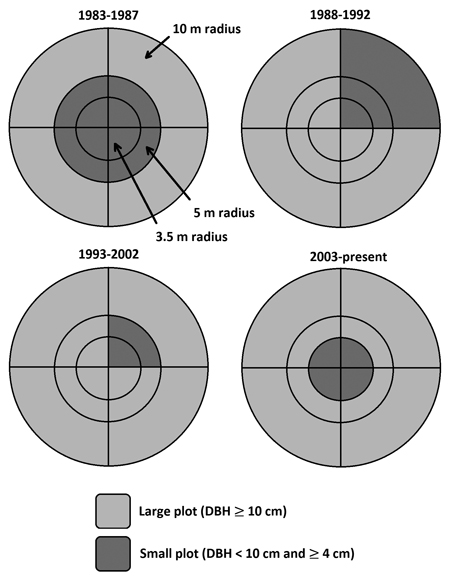
Fig. 1. Permanent plot design for Swedish national forest inventory (NFI) from 1983 to present day. Large plot = all trees with a diameter at breast height (DBH, 1.3 m) ≥ 10 cm was measured with callipers. Small plot = all trees with a DBH < 10 cm and ≥ 4 cm was measured with callipers.
The long-term forest experiment data consisted of permanent plots in Scots pine, and Norway spruce dominated stands used for experiments on stand establishment, spacing, and thinning (Elfving and Kiviste 1997; Nilsson et al. 2010). The stand history is well documented in most cases, and plots are regenerated through planting, direct seeding, or natural regeneration. Because the experiments are more carefully managed, they are more homogeneous than the average production forest in the NFI data, both in terms of species composition and structure. The plot size varied between 0.02 ha and 0.2 ha (0.06 ha on average).
For the basal area growth and yield models for Scots pine (Model 1) and Norway spruce (Model 2), yield data or total basal area (m2 ha–1) was used from both the Swedish long-term experiments between 1960 and 2017, and Swedish NFI between 1993 and 2017 (Table 1). This was possible because this modelling approach allows for various growth period lengths. Including measurements with different interval lengths should result in a model that makes better long-term projections (Lee 1998). The used period lengths were 5 to 20 years for the Swedish NFI data and 1 to 36 years for the long-term experiment data. Because total production (including self-thinning and removals in thinnings) was modelled in Model 1 and Model 2, only permanent plots with at least one measurement before the first thinning were used for model fitting of Model 1 and Model 2. Thus, 836 (4623 periods) Norway spruce plots and 1922 (7798 periods) Scots pine plots were used.
For the basal area growth models for Scots pine (Model 3) and Norway spruce (Model 4), five-year basal area growth (m2 ha–1 5-years–1) of all living trees present at the beginning and end of the period was used. Data came from NFI permanent plots measured from 2003 to 2017 (Table 1). These were remeasured on 5-year intervals and had a consistent plot size and layout (Fig. 1). There was a total of 2130 (3286 periods) Norway spruce plots and 3088 (4961 periods) Scots pine plots. The new growth models were inspired by Elfving’s growth model currently used in the Swedish forest planning system Heureka (Elfving 2010; Wikström et al. 2011). The new growth models were created using newer data to see if models based on NFI data from the 2000s performed differently from Elfving’s model using NFI data from the 1980s.
For model comparison, an independent data set was used (GG) consisting of 20 sites (10 Scots pine and 10 Norway spruce) from a thinning and fertilisation experiment established 1966–1983 (Nilsson et al. 2010). The experimental plots were established at the time of first thinning when the top height was 12–18 m. The experiment consisted of pure stands of Norway spruce and Scots pine. The Norway spruce stands were located in southern and central Sweden (56.1°N–63.1°N), and the Scots pine stands were located from the county of Scania in the south to Norrbotten in the north (56.2°N–67.3°N) (Fig. 2). The plot size was 0.1 ha on average. The treatments that were applied were different thinning and fertilisation treatments. After establishment, plots were remeasured at each thinning and occasionally in between. The plots used in this study came from two treatments. Treatment A, included 3 to 6 thinnings with a mean thinning grade of 22% for Norway spruce, and 3 to 4 thinnings with a mean thinning grade of 26% for Scots pine. Treatment I was the untreated control. These treatments were chosen because models should be tested on both unmanaged and managed forests. These treatments were also the most common among the different sites and had long growth records.
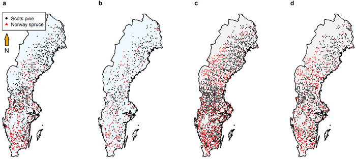
Fig. 2. Locations of the plots used for model fitting and validation for (a) growth and yield model fitting (Model 1 and Model 2; 1288 Scots pine plots and 552 Norway spruce), (b) growth and yield model validation (Model 1 and Model 2; 634 Scots pine and 284 Norway spruce), (c) growth model fitting (Model 3 and Model 4; 2059 Scots pine and 1422 Norway spruce), and (d) growth model validation (Model 3 and Model 4; 1029 Scots pine and 708 Norway spruce).
2.2 Data management and selection
Data were sorted and processed before model fitting. In the long-term experiment, the only necessary pre-processing was adjusting basal area increment to the time of the year the plots were measured in different revisions (see details below) and removing outlier plots. The outlier plots had either negative or extremally high (around three times) total basal area development compared to the growth trends of plots with similar stand and site conditions in the data. In contrast, the NFI data were in tree list form and needed rigorous sorting and management before model fitting. Here follows a description of the steps used to process the NFI data.
Age was not measured for every callipered tree but was estimated on a plot level by coring two trees outside the 10 m radius permanent plot. The cored trees had a DBH as close to the quadratic mean diameter of the plot as possible. These age estimates were not always consistent between measurements. Therefore, it was necessary to compute an age that was consistent with time between measurements. The new age was calculated for each plot by taking every plot age from each measurement and calculating backwards to when the plot was first measured. The age at first measurement (Ai) for individual plots was calculated using the following equation:
![]()
where A is estimated plot mean age, Ym was year of measurement, and Yi was year of initial measurement. Age at first measurement was calculated for every plot measurement resulting in a maximum of six Ai values for each plot. An average of the backtracked ages was created and set as the initial age of the plot when it was first measured (agestart):
![]()
where n is the number of estimated ages per plot. To get the age at a particular time, the number of years from the plot’s agestart was added. For example, a plot first measured in 1983 yielded an agestart of 23. The age in 2003 would then be 23 + 20 = 43 years.
Because plots were not measured consistently at the same time of the year, growth needed to be adjusted between two measurements to the actual period length. For example, if a plot was measured in spring 2003 and late summer 2008, the real number of growing seasons was closer to six than five. An adjustment to account for the different measurement timings was applied by calculating how far into the growing season the measurements were made by estimating the completion of annual rings using the following equation (Elfving 2010):
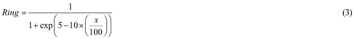
where Ring is the degree of completion of an annual growth ring when the measurement was made (0 < Ring < 1) and x is the number of days past the growing season’s start. Regardless of location, the ring growth season was assumed to last 100 days (i.e. May 20 to August 29) (Valinger 1992; Soderberg et al. 1993; Elfving 2010). Ring was computed in both measurement years, and growth was adjusted so that the number of growing seasons would match the number of years between measurements. For example, if recorded growth was 6 m2 ha–1 during 5.4 growth seasons between 2003 and 2008, the adjusted growth for five seasons would be (6/5.4)×5 = 5.56 m2 ha–1. This adjustment was done for the NFI and long-experiment data.
There was also an issue with ingrowth for the NFI plots caused by the inventory design (Fig. 1), where trees with a DBH below 10 cm were being measured in a smaller plot compared to trees with a DBH equal or larger than 10 cm. This resulted in trees suddenly appearing in the large plot (ingrowth), causing artificial jumps in basal area. We addressed this issue by using the trees present at the end of the period with a diameter larger than 10 cm to predict diameter at the beginning of the period when the diameter was smaller than 10 cm. These functions estimated diameter at the beginning of the period based on diameter at the end of the period, age, and site index. Using this method, trees that grew into the larger size class by the end of the period that were not measured in the small plot were assigned a diameter at the beginning of the period. Basal area was then calculated by summing basal area of trees with DBH larger than 10 cm measured in the big plot, DBH between 4 and 10 cm measured in the small plot, and DBH between 4 and 10 cm estimated in the big plot.
A further issue related to ingrowth was trees growing from a DBH below 10 cm to a DBH equal to or larger than 10 cm during a growth period. This initially caused both artificial increases and decreases in basal area because the same tree would be divided by a different plot area when calculating basal area per ha (m2 ha–1). To avoid these problems, the plot area a tree had at the end of the period was used to calculate its basal area per ha at the period’s start as well.
Plot thinning was inferred from harvested trees. First, basal area of the harvested trees before removal was calculated. This basal area was then compared to the total basal area before thinning to get a thinning grade (percent of initial basal area removed, Gremoved/Gbefore). The thinning grade was compared to the NFI’s stand management classification to select the removals resulting from thinning. The comparison showed that most removals classified as thinning had a removal between 10 and 60%, with a 35% mean. The removals were also compared to natural mortality and final felling, which mainly occurred below 10% and above 60%, respectively. From this analysis, removals over 60% were classified as harvest/final felling and below 10% as no management/natural mortality. Removals larger or equal to 10% and lower or equal to 60% were classified as thinnings.
Not all the available data were used in the model fitting process. Instead, the model fitting was restricted to plots where, at the beginning of the period;
- The proportion of basal area was ≥ 70% of either Norway spruce or Scots pine with no restrictions on the remaining 30%
- Mean tree height ≥ 5 m
- Plot age ≥ 10 years
- No harvest during the current or two previous growth periods
There were also specific restrictions for each model on top of these general restrictions used for both the Swedish NFI and long-term experiment data. For the growth models (Model 3 and Model 4), no thinning was allowed during the five-year growth period. The reason was that the five-year growth should be the total growth of all living trees present at the beginning and end of the period. For Model 1 and Model 2 using total basal area, the selected plots had a height below 10 m the first time they were measured. This height restriction allowed for a more accurate total basal area production.
2.3 Modelling
2.3.1 Compatible growth and yield model
When fitting the compatible growth and yield models (Model 1 and Model 2), two-thirds of the selected data was used for model fitting, and the rest was used for model validation. The best fit for both Scots pine and Norway spruce came with the Schumacher 2 polymorphic function (Schumacher 1939). The shape of the Schumacher equation was augmented by initial plot stem number before thinning to account for the effect of stem density on basal area development:

where G2 is basal area (m2 ha–1) at period end, G1 is basal area (m2 ha–1) at period start, t1 is age at period start, t2 is age at the end of the period, and ST is initial stem number (stems ha–1) before thinning, a, b, and c are parameters to be estimated, and log is the natural logarithm. The best model was chosen by analysing normality and bias of the residuals and minimising root mean square error (RMSE). To reduce the effect of autocorrelation, parameter significance was checked by fitting the models to a random sub-sample containing one interval per plot. The models were fitted using the nls, nls2, or nlsLM functions in R, from the lme4, nls2 (Grothendieck 2013), and minpack.lm (Elzhov et al. 2016) packages. All modelling and statistics in this study were computed with the statistical software R (version 3.6.1) (R Core Team 2016). Model validation was done by predicting basal area using the one-third validation data (Table 1) and comparing precision and bias of predicted basal area against the observed basal area.
2.3.2 Growth models
The selected data were randomly divided into two-thirds for model fitting and one-third for model validation when fitting Model 3 and Model 4. Linear mixed effects models were used in the lme4 package (Bates et al. 2015), when determining variable significance to account for the random effects of site because of multiple measurements on each site. Only significant variables were kept in the final models, and VIF values were evaluated to exclude variables with severe collinearity with other variables (VIF > 10). We used the lmerTest package (Kuznetsova et al. 2017) to generate p-values for the lmer output, and the MuMIn package (Barton, 2018) to calculate R2 for the mixed models. Some variables were transformed using scaled power transformations (Cook and Weisberg 1999) to improve linearity and fulfil the assumptions of normality and homoscedasticity. To find the best transformations, the distributions of the independent variables were analysed using the SPTLambda function in R. Since the response variables were log-transformed using the natural logarithm, the models needed to be corrected for transformation bias (Vanclay and Skovsgaard 1997). The correction factor from Baskerville (1972) accounted for this bias. Variables used in the final growth models (Eq. 5) are presented in Table 2. The validation of the models was done by predicting basal area growth using the one-third validation data (Table 1) and comparing precision and bias of predicted growth against observed growth.
![]()
where Y is the dependent variable log(G_growth), the natural logarithm of basal area growth over five years (m2 ha–1 5-years–1), b0 is intercept, b1–bk is estimated coefficients (Table 5), x1–xk is independent variables (Table 2), and ε is model error.
| Table 2. Definition of variables used in model fitting and validation. Model 1 = basal area growth and yield model (m2 ha–1) for Scots pine in Sweden, Model 2 = basal area growth and yield model (m2 ha–1) for Norway spruce in Sweden, Model 3 = basal area growth model (m2 ha–1 5-years–1) for Scots pine in Sweden, and Model 4 = basal area growth model (m2 ha–1 5-years–1) for Norway spruce in Sweden. | ||
| Variable | Definition | Included in model |
| t1 | Age at period start (year) | Model 1, Model 2, Model 3, Model 4 |
| t2 | Age at period end (year) | Model 1, Model 2 |
| ba | Basal area at period start (m2 ha–1) | Model 3, Model 4 |
| G1 | Total basal area at period start (m2 ha–1) | Model 1, Model 2 |
| G2 | Total basal area at period end (m2 ha–1) | Model 1, Model 2 |
| stem | Stem number (stems ha–1) at the start of the period | Model 3, Model 4 |
| ST | Initial stem number (stems ha–1) before thinning | Model 1, Model 2 |
| veg | Ground vegetation type index (Table 3) | Model 3, Model 4 |
| thinn1 | The thinning grade (Gout/Gbefore) of a thinning performed one period ago. Gout = removed basal area in thinning. Gbefore = basal area before thinning | Model 3, Model 4 |
| thinn2 | The thinning grade (Gout/Gbefore) of a thinning performed two periods ago | Model 3, Model 4 |
| propspruce | Norway spruce proportion of the total basal area (0–1) | Model 3, Model 4 |
| moist | 1 if the soil moisture class is classified as moist, else 0 | Model 4 |
| tsum | Temperature sum(day-degrees > 5 °C), calculated from altitude and latitude (Odin et al. 1983), divided by 1000 | Model 3, Model 4 |
| peat | 1 if the soil is classified as peat, else 0 | Model 3 |
| depthind | 1 if the soil depth is <=0.5 m, else 0 | Model 3 |
To get an indicator of site fertility, a vegetation index was used (veg-index). This index was based on the Swedish NFI vegetation-type classification and ranged between –5 and +4 (Elfving 2010). Each vegetation class is given an index that reflects site fertility (Table 3).
| Table 3. Ground vegetation type index (veg) variable definition. Veg-type was the classification use by the Swedish NFI and the veg-index is the veg variable used in Model 3 = basal area growth model (m2 ha–1 5-years–1) for Scots pine in Sweden, and Model 4 = basal area growth model (m2 ha–1 5-years–1) for Norway spruce in Sweden. | ||
| Veg-type classification (Swedish) | Veg-type classification (English) | Veg-index |
| Högört utan ris | Rich-herb without shrubs | 4 |
| Högört med ris/blåbär | Rich-herb with shrubs/bilberry | 2.5 |
| Högört med ris/lingon | Rich-herb with shrubs/lingonberry | 2 |
| Lågört utan ris | Low-herb without shrubs | 3 |
| Lågört med ris/blåbär | Low-herb with shrubs/bilberry | 2.5 |
| Lågört med ris/lingon | Low-herb with shrubs/lingonberry | 2 |
| Utan fältskikt | No field layer | 3 |
| Bredbl. gräs | Broadleaved grass | 2.5 |
| Smalbl. gräs | Thinleaved grass | 1.5 |
| Carex ssp.,Hög starr | Sedge, high | –3 |
| Carex ssp.,Låg starr | Sedge, low | –3 |
| Fräken | Horsetail, Equisetum ssp. | 1 |
| Blåbär | European blueberry, bilberry | 0 |
| Lingon | Lingonberry | –0.5 |
| Kråkbär | Crowberry | –3 |
| Fattigris | Poor shrub | –5 |
| Lavrik | Lichen, frequent occurrence | –0.5 |
| Lav | Lichen, dominating | –1 |
2.4 Model comparison
In the model comparison, the new models created in this study were applied to an independent data set. The main basal area growth model (Elfving) used in Heureka was also included in the model comparison. The Elfving model is a linear regression model predicting 5-year basal area growth (m2 ha–1 5-years–1) for stands of Scots pine, Norway spruce, and silver birch (Betula pendula Roth) in all of Sweden. It was developed using permanent plots from the Swedish NFI, first measured 1983–1987 and then remeasured 5 years later, 1988–1992. The parameters included in the model are presented in the appendix (Supplementary file A1: Table A.1). For more information about the model, see Elfving (2010).
Model comparison was performed by running the models from the first measurement and the following five growth periods. The models were used to estimate total basal area (m2 ha–1), including mortality and thinning removals. Since net basal area was used in Model 3, Model 4, and the Elfving model, mortality was estimated using the mortality function from Siipilehto et al. (2020). The length of model comparison was different for different plots, with 34–40 years for Scots pine and 27–34 years for Norway spruce (Table 1). The period lengths varied between 2 to 14 years (average 7 years) and 3 to 11 (average 6 years) respectively. For Scots pine, measurements came from between 1969 and 2015, and for Norway spruce, between 1966 and 2007. The different models were compared using residual analysis to determine the precision and bias of predictions.
3 Results
3.1 Model fitting
The fitted growth and yield models showed a good and relatively unbiased fit against the NFI data with similar patterns for both species when plotted against fitted basal area (Fig. 3 and 4) and other predictor variables (Suppl. file A1: Fig. A.1 and A.2). The Scots pine model (Model 1) had a better fit (RMSE (m2 ha−1) = 1.404) to its data compared to the model for Norway spruce (Model 2; RMSE = 2.507) (Table 4). The validation showed good and relatively unbiased residuals when plotted against predicted basal area (Fig. 3 and 4) and other predictor variables (Suppl. file A1: Fig. A.1 and A.2). When comparing the species-specific models, Model 2 shows a higher basal area growth for comparable stand basal area and age (Fig. 5.)
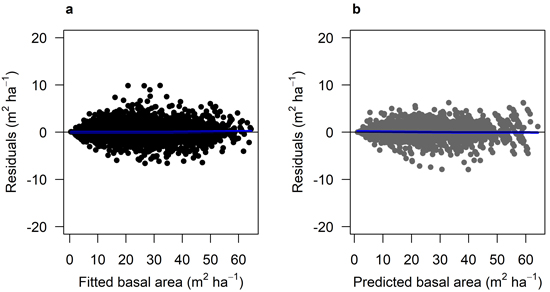
Fig. 3. Residual basal area for Model 1 (Scots pine). a) residuals for the fitted model against fitted basal area (m2 ha–1) using data set M1F, with data from the Swedish national forest inventory and long-term experiments. b) residuals for the model validation against predicted basal area (m2 ha–1) using data set M1V, with data from the Swedish national forest inventory and long-term experiments. The blue lines show the trend in the residuals.
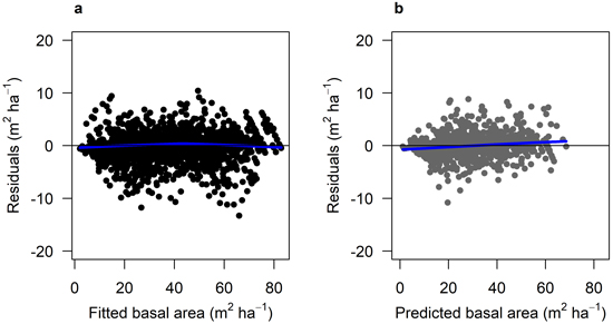
Fig. 4. Residual basal area for Model 2 (Norway spruce). a) Residuals for the fitted model against fitted basal area (m2 ha–1) using data set M2F, with data from the Swedish national forest inventory and long-term experiments. b) residuals for the model validation against predicted basal area (m2 ha–1) using data set M2V, with data from the Swedish national forest inventory and long-term experiments. The blue lines show the trend in the residuals.
| Table 4. Estimated parameters for the growth and yield models and model root mean squared error (RMSE; m2 ha–1) for Scots pine (Model 1) and Norway spruce (Model 2) in Sweden. All estimated parameters were significant at p < 0.05. | ||||||
| Model | RMSE (m2 ha–1) | a | b | c | ||
| Model 1 | Fitted model | 1.404 | Estimate | 4.822 | 0.151 | 0.224 |
| SE | 0.017 | 0.007 | 0.007 | |||
| Validation | 1.472 | |||||
| Model 2 | Fitted model | 2.507 | Estimate | 5.113 | 0.328 | 0.119 |
| SE | 0.018 | 0.022 | 0.009 | |||
| Validation | 2.279 | |||||
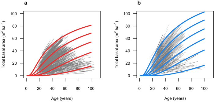
Fig. 5. Predicted total basal area (m2 ha–1) over age (years). a) red lines show Model 1 (Scots pine) when basal area is 65, 50, 35, 20 and 5 m2 ha–1 at 60 years. Light grey lines represent model fitting data (M1F), and dark grey lines represent validation data (M1V). Initial stem number was set to 2000 stems ha–1. b) blue lines show Model 2 (Norway spruce) when basal area is 80, 65, 50, 35, 20 and 5 m2 ha–1 at 60 years. Light grey lines represent model fitting data (M2F), and dark grey lines represent validation data (M2V). Initial stem number was set to 2000 stems ha.
The growth models for Scots pine (Model 3) and Norway spruce (Model 4) contained similar explanatory variables (Table 5). The most important variables were age at the beginning of the period (age1), basal area at period start (ba), and ground vegetation class (veg). The residual plots of the two growth models where the residuals were plotted against fitted basal area growth (Fig. 6 and 7) and other predictor variables (Suppl. file A1: Fig. A.3 and A.4) showed a good and relatively unbiased fit. The validation showed a similar pattern to the model fitting for both growth models when plotted against predicted basal area (Fig. 6 and 7) and other predictor variables (Suppl. file A1: Fig. A.3 and A.4).
| Table 5. Statistical output of basal area growth models for Scots pine (Model 3) and Norway spruce (Model 4) in Sweden. The response variable was log(G_growth), the natural logarithm of basal area growth over five years (m2 ha–1 5-years–1). The variable exponents were selected to improve variable normality. R2 is the marginal r-square, i.e., a measure of the explanatory power of the fixed effects only. Site was set as random effect. | |||||||
| Model | Coefficient | Estimate | Std. Error | Pr(>|t|) | RMSE | R2 | Random variance |
| Model 3 (Scots pine) | Intercept | 1.547 | 1.260e-01 | < 2e-16 | 0.24 | 0.70 | |
| age10.2 | –1.579 | 3.660e-02 | < 2e-16 | ||||
| ba0.6 | 1.036e-01 | 6.013e-03 | < 2e-16 | ||||
| stem0.2 | 4.105e-01 | 1.745e-02 | < 2e-16 | ||||
| veg | 3.493e-02 | 4.590e-03 | 2.71e-14 | ||||
| thinn10.1 | 2.900e-01 | 1.898e-02 | < 2e-16 | ||||
| thinn20.1 | 2.231e-01 | 1.928e-02 | < 2e-16 | ||||
| peat | –2.808e-01 | 2.519e-02 | < 2e-16 | ||||
| depthind | –5.444e-02 | 1.947e-02 | 0.00470 | ||||
| tsum | 4.417e-01 | 3.422e-02 | < 2e-16 | ||||
| propspruce | 2.898e-01 | 9.098e-02 | 0.00121 | ||||
| Site (random) | 9.245 e-02 | ||||||
| Model 4 (Norway spruce) | Intercept | 5.402e-01 | 1.931e-01 | 0.005195 | 0.29 | 0.69 | |
| age10.25 | –9.577e-01 | 3.531e-02 | < 2e-16 | ||||
| ba0.74 | 5.011e-02 | 3.021e-03 | < 2e-16 | ||||
| stem0.2 | 4.175e-01 | 1.883e-02 | < 2e-16 | ||||
| veg | 8.257e-02 | 5.669e-03 | < 2e-16 | ||||
| thinn12 | 2.014 | 1.704e-01 | < 2e-16 | ||||
| thinn22 | 1.269 | 1.964e-01 | 1.18e-10 | ||||
| propspruce | 3.419e-01 | 9.095e-02 | 0.000175 | ||||
| moist | –1.228e-01 | 4.532e-02 | 0.006770 | ||||
| tsum | 4.032e-01 | 4.340e-02 | < 2e-16 | ||||
| Site (random) | 7.072e-02 | ||||||
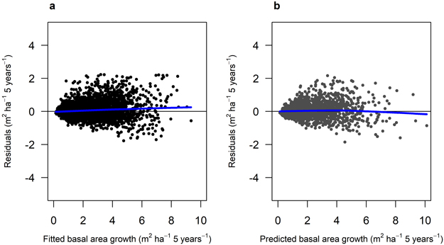
Fig. 6. Residuals for Model 3 (Scots pine). A) residuals for the fitted model against fitted basal area growth (m2 ha–1 5 years–1) using data set M3F, with data from the Swedish national forest inventory. b) residuals for the model validation against predicted basal area growth (m2 ha–1 5 yrs–1) using data set M3V, with data from the Swedish national forest inventory. The blue lines show the trend in the residuals.
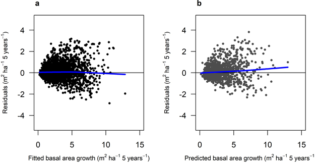
Fig. 7. Residuals for Model 4 (Norway spruce). a) residuals for the fitted model against fitted basal area growth (m2 ha–1 5 years–1) using data set M3F, with data for the Swedish national forest inventory. b) residuals for the model validation against predicted basal area growth (m2 ha–1 5 yrs–1) using data set M4V, with data from the Swedish national forest inventory. The blue lines show the trend in the residuals.
3.2 Model comparison
The models showed relatively similar results when tested against the independent experiment data (Fig. 8). The Scots pine models had better predictions over time with lower RMSE (m2 ha−1) than the Norway spruce models (Table 6). On average, across all five periods, the RMSE for the Scots pine models was 2.204 for Model 1, 1.708 for Model 3, and 2.266 for Elfving. For Norway spruce, the average RMSE was 4.156 for Model 2, 5.228 for Model 4, and 4.188 for Elfving.
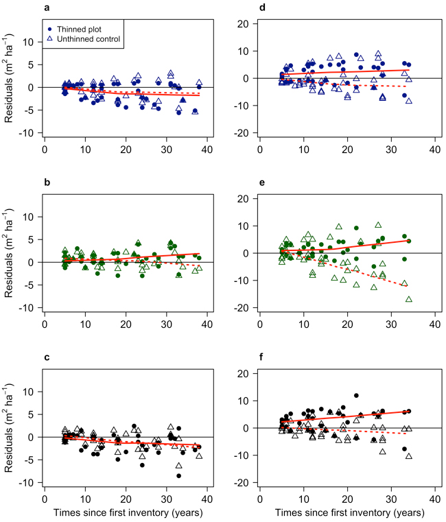
Fig. 8. Residual modelled basal area relative to independent data from the GG experiment as a function of time since first measurement. Plots a, b and c are Scots pine (using the GGpine data set, with data from a Swedish long-term thinning and fertilisation experiment), and d, e and f are Norway spruce (using the GGspruce data set, with data from a Swedish long-term thinning and fertilisation experiment). Plot a (Model 1) and d (Model 2) show residuals for the growth and yield models. Plot b (Model 3) and e (Model 4) show residuals for the growth models. Plots c and f show residuals for Elfving’s model used on Scots pine (GGpine) (c) and Norway spruce (GGspruce) (f). The solid red lines show the trend in the residuals for the thinned plots, and the dotted lines the residual trend for the unthinned plots.
| Table 6. Mean residual bias (%) and root mean squared error (RMSE) for each model and growth period (average 7 years for Scots pine and 6 years for Norway spruce), compared against independent data (GGpine and GGspruce). Model 1 = basal area growth and yield model (m2 ha–1) for Scots pine, Model 2 = basal area growth and yield model (m2 ha–1) for Norway spruce, Model 3 = basal area growth model (m2 ha–1 5-years–1) for Scots pine, Model 4 = basal area growth model (m2 ha–1 5-years–1) for Norway spruce, and Elfving = basal area growth model (m2 ha–1 5-years–1) for Scots pine, Norway spruce, and silver birch. | |||||||||||
| Species | Model | Mean residual bias % (SE) | RMSE (m2 ha–1) | ||||||||
| Period | Period | ||||||||||
| 1 | 2 | 3 | 4 | 5 | 1 | 2 | 3 | 4 | 5 | ||
| Scots pine | Model 1 | 0.35 (0.60) | –1.49 (0.98) | –3.00 (1.28) | –2.44 (1.67) | –7.17 (1.66) | 0.70 | 1.43 | 2.15 | 2.75 | 3.99 |
| Model 3 | 2.55 (0.74) | 1.98 (0.99) | 2.10 (1.12) | 3.58 (1.54) | –1.62 (1.20) | 1.08 | 1.45 | 1.81 | 2.49 | 1.71 | |
| Elfving | 0.92 (0.66) | –1.94 (1.14) | –3.46 (1.25) | –3.77 (1.40) | –8.38 (1.82) | 0.8 | 1.66 | 2.12 | 2.51 | 4.24 | |
| Norway spruce | Model 2 | 0.86 (1.35) | 0.93 (1.63) | 0.78 (1.95) | –0.95 (2.23) | –1.62 (2.73) | 2.32 | 3.32 | 4.29 | 5.30 | 5.55 |
| Model 4 | 1.34 (1.44) | 0.12 (1.92) | –1.04 (2.24) | –3.37 (2.79) | –2.59 (3.35) | 2.36 | 3.81 | 4.98 | 7.1 | 7.9 | |
| Elfving | 2.14 (1.32) | 2.50 (1.58) | 2.023 (1.76) | –0.25 (2.15) | –1.12 (2.83) | 2.4 | 3.44 | 4.19 | 5.28 | 5.64 | |
For Scots pine, Model 3 and Elfving model showed a tendency to overestimate basal area more over longer times. The residual bias was on average –7.17% and –8.38% respectively in the final period (period 5), compared to –1.65% for Model 3 (Table 6). For Norway spruce, the models were relatively unbiased with time, where the bias on average the final period (period 5) was –1.62% for Model 2, –2.59% for Model 4, and –1.12 for Elfving (Table 6).
All models also showed an increased spread of residuals with less accurate predictions at the end of the comparison. The largest increase in variation was for Model 4 which increased RMSE from 2.36 in the first period to 7.90 in the final period.
4 Discussion
4.1 Model comparison: all models had similar performance
Altogether, there were no clear differences between the predictions of different models and no clear patterns in when the models worked better or worse. Expected benefits of long-term precision using compatible growth and yield models (Model 1 and Model 2), like path invariance and variable period length (Clutter 1963; Weiskittel et al. 2011), could not be seen for these plots and periods, regardless of plot treatment and location. Perhaps a longer comparison period than 30–40 years could have shown clearer results for the model comparison. Also, the current basal area model used in Heureka (Elfving) works well, even compared to species-specific models using new data and different equations. The lack of differences makes it difficult to say that one model was constantly better. However, the results illustrate the power of the relatively simple Model 1 and Model 2, which only used age, basal area, and initial stem number as input variables. Even though these growth and yield models did not show a more stable prediction with time, they include other strengths such as choosing period length and simple input variables. Choosing period lengths makes these models more flexible and easier to use than fixed five-year growth models such as those used in this study (Model 3, Model 4, and Elfving). The simple input variables make the growth and yield models a good alternative for predicting stand development in managed forests where age is known and basal area and stem number are estimated through remote sensing (Nilsson et al. 2017). If the initial stem number before thinning is unavailable, the average initial stem numbers from this study could be used. These are 1544 stems ha–1 (SE = 11.2) for Scots pine and 2380 stems ha–1 (SE = 16.1) for Norway spruce.
Comparison of the models against independent data showed that the ability of the models to predict basal area development was good. However, precision and bias varied both with time and model. For Scots pine, Model 3 had the best long-term precision and minimally underestimated basal area (2 to 3%). Model 1 and Elfving model tended to overestimate with time, especially in the final period where basal area was overestimated by 6 and 8%, respectively. A reason for the more apparent overestimation bias for the Elfving model could be due to that model being the same for Scots pine and Norway spruce. Studies like Eko et al. (2008) have shown that Norway spruce stands have higher production than Scots pine in Swedish NFI data. This was also shown in this study where Norway space models had a higher growth compared to models developed for Scots pine dominated stands (Fig. 5). In the Elfving model, this species difference was captured with the species proportion of basal area where plots with more Scots pine grew slower (Elfving, 2010). This species adjustment was, however, insufficient for the plots used in this comparison.
The models for Norway spruce differed somewhat in their ability to predict basal area. Both Model 2 and Elfving’s model showed a similar and unbiased ability to predict basal area over time. In contrast, Model 4 had a more substantial residual variation and a large overestimation for some plots. The plots with considerable overestimation in the later stages were primarily unthinned control plots. This indicates that growth of Model 4 did not flatten off as aggressively as these experimental plots and other tested models did. Another reason may be that the estimations for these overestimated control plots were already biased after 10-year predictions (Fig. 8). By running the model for a long time using these biased estimations, errors accumulate as predictions were made from increasingly biased previous predictions (Holm 1981; Kangas 1997). Predictions by both Elfving and Model 2 model had increased RMSE between the first and last periods, but not to the same extent and with less bias.
The included variables in the Model 3 and Model 4 models were quite similar. The variables that did not occur in both models were connected to the species availability in the Swedish NFI data set. For example, plots with peat and shallow soils only occurred to a large extent where Scots pine was dominant. Therefore, these variables became significant and included in the final Model 3. The moist variable worked the same way in the Norway spruce model (Model 4), where a large portion of the Norway spruce dominated plots were classified as moist.
4.2 Limitations imposed by data collection design
We used NFI data for the Model 3 and Model 4 models because these five-year growth models required a consistent five-year interval. Also, one of the objectives was to see if data from between 2003 and 2017 would result in different model performance than the Elfving model based on data from the 1980s. The growth and yield models (Model 1 and Model 2) allowed combining data from both NFI and long-term experiments, despite different period lengths. The different period lengths of the experimental data needed a type of equation that could deal with this inconsistency both within and between experiments. It was, therefore, suitable for the growth and yield models but not for the five-year growth models. Another reason for including the experimental data when fitting Model 1 and Model 2 was that yield data on total basal area production was used for these models. The long-term experiment data contained older and more accurate records on total basal area production than the Swedish NFI data and was therefore included.
The data collection design was the likely source of uncertainty in model predictions. Age was a complicated variable in this study and is a weakness of using the Swedish NFI for growth and yield model development (Fahlvik et al. 2014). The problem was that age was not measured for each plot but rather estimated. This is a problem because the estimated age varied between periods. The age usually increased by fewer or more years than it should have. For example, some plots with an age of 60 years in 1983 were recorded as 65 years old in 1993, ten years later. Our solution was to take the average of all estimates since we could not know which ones were reliable. As discussed in Elfving (2010), it may have been desirable to avoid age as a variable, but that was not easy since age explained much of the variation in basal area development. All this uncertainty added to the error and overall uncertainty of the models.
Different plot sizes for different sized trees are understandable in an inventory system for logistical reasons, to reduce the number of trees to be measured. But the smaller plot used to measure trees between 4 and 9.9 cm was not entirely representative of the whole 10 m plot and resulted in ingrowth. We dealt with ingrowth by estimating the basal area of small trees in the whole 10 m radius plot. The plot basal area was then made up of trees with DBH over 10 cm measured in the large plot, trees between 4 and 10 cm measured in the small plot, and trees between 4 and 10 cm estimated outside the small plot. The resulting basal area was then partly a prediction of previous basal areas. This was still a better option than the sometimes severe basal area growth overestimation caused by ingrowth. A similar issue occurred when the Swedish NFI plot area changed between inventories. This also caused problems with ingrowth and difficulties with growth analysis. Plot size issues are good illustrations of the problems that arise when making changes to long-term permanent plot inventories. The Swedish NFI realised this at the beginning of the 2000s and worked to standardise the inventory (Fridman et al. 2014), but the previous changes still cause problems.
Another limitation on the models was the rarity of older forests in the available data for model construction. The main reason for this was that forests above 100 years are not common in Sweden and made up a small part of the final datasets after applying the restrictions. This was especially true for Model 1 and Model 2. One of the restrictions when selecting data was that a plot could not be taller than 10 m at first measurement to ensure accurate total basal area production estimations. The models should therefore be used with caution on old forests over 100 to 150 years old.
4.3 Prospects for use of growth and yield models
The models created in this study were developed for relatively pure stands of Norway spruce and Scots pine (≥70% of basal area). However, according to the Swedish NFI data, around 30% Swedish forests are not so homogenous. Therefore, there is a need for models that can take mixture effects into account, especially when including other species than Norway spruce and Scots pine. Using the Swedish NFI, models for mixed forests could probably be developed for common species like Scots pine, Norway spruce, and silver birch. Making models for other species may be more difficult since they occur infrequently in the data and with a large geographical variation. For those species, plots in long-term experiments are necessary. However, these experiments may have the same problem representing geographical variation and variation in site properties.
The minor differences between the models evaluated in this study suggest that other approaches than purely statistical forest growth and yield models are needed to improve the models’ site adjustment and ability to make accurate long-term predictions, even during changes in growth conditions. This could be achieved by developing hybrid physiological/mensurational models where climate effects on production are included (Mason et al. 2007).
5 Conclusions
In this study, compatible growth and yield models and growth models, predicting stand basal area, were developed for Scots pine and Norway spruce. In the long-term model comparison, there were no apparent differences between the models developed in this study and the one currently used in Heureka in their ability to predict basal area development. The theoretically beneficial features of compatible growth and yield models, like path invariance, did not give any advantages in the model comparison against the independent data. However, their ability to predict basal area development despite their simplicity illustrates the power of this method of forest growth and yield modelling. This makes it a good alternative when data availability is limited. Also, there were no clear differences between the new and old growth models despite more and newer data in the models from this study. The lack of differences means that the basal area growth model used in Heureka can continue to be used. The future development of growth and yield models should focus on forests with heterogeneous species composition, age, and tree size. These forests are common and may become even more so in the future, but there is a lack of models for this type of forests. Future studies should also investigate ways to better incorporate site properties and weather into growth and yield models to better deal with short- and long-term changes in temperature and precipitation.
Acknowledgements
The authors gratefully acknowledge the entire team at the Swedish National Forest Inventory and Unit for Field-based Forest Research, SLU, for providing field data and support.
Funding
Funding for this work was provided by the research program Trees and Crops for the Future (TC4F) and the Swedish Research Council for Sustainable Development (FORMAS) under grants 2018-00968 and 2018-01820.
Declaration of openness of research materials, data, and code
The datasets and the custom R-code for model development and analysis are available upon reasonable request by contacting the corresponding author.
Authors’ contributions
MG, UN, and EM developed the research idea and methodology. MG led the work with data analysis, model development, and manuscript writing, with valuable support from UN, EM, and GV.
References
Bailey RL, Ware KD (1983) Compatible basal-area growth and yield model for thinned and unthinned stands. Can J Forest Res 13: 563–571. https://doi.org/10.1139/x83-082.
Baskerville GL (1972) Use of logarithmic regression in the estimation of plant biomass. Can J Forest Res 2: 49–53. https://doi.org/10.1139/x72-009.
Bates D, Machler M, Bolker BM, Walker SC (2015) Fitting Linear Mixed-Effects Models Using lme4. J Stat Softw 67: 1–48. https://doi.org/10.18637/jss.v067.i01.
Buckman RE (1962) Growth and yield of red pine in Minnesota. Technical Bulletin 1272.
Clutter JL (1963) Compatible growth and yield models for loblolly pine. Forest Sci 9: 354–371. https://doi.org/10.1093/forestscience/9.3.354.
Cook RD, Weisberg S (1999) Applied regression including computing and graphics. John Wiley and Sons, New York. https://doi.org/10.1002/9780470316948.
Eko PM (1985) En produktionsmodell för skog i Sverige, baserad på bestånd från riksskogstaxeringens provytor. [A growth simulator for Swedish forests, based on data from the national forest survey]. Swedish University of Agricultural Sciences, Department of Silviculture. ISBN 91-576-2386-4.
Eko PM, Johansson U, Petersson N, Bergqvist J, Elfving B, Frisk J (2008) Current growth differences of Norway spruce (Picea abies), Scots pine (Pinus sylvestris) and birch (Betula pendula and Betula pubescens) in different regions in Sweden. Scand J Forest Res 23: 307–318. https://doi.org/10.1080/02827580802249126.
Elfving B (2010) Growth modelling in the Heureka system. Swedish University of Agricultural Sciences, Faculty of Forestry.
Elfving B, Kiviste A (1997) Construction of site index equations for Pinus sylvestris L. using permanent plot data in Sweden. Forest Ecol Manag 98: 125–134. https://doi.org/10.1016/S0378-1127(97)00077-7.
Elzhov TV, Mullen KM, Spiess A, Bolker B (2016) minpack.lm: R Interface to the Levenberg-Marquardt nonlinear least-squares algorithm found in MINPACK, plus support for bounds. https://cran.r-project.org/package=minpack.lm.
Fahlvik N, Elfving B, Wikstrom P (2014) Evaluation of growth models used in the Swedish Forest Planning System Heureka. Silva Fenn 48, article id 1013. https://doi.org/10.14214/sf.1013.
Fridman J, Holm S, Nilsson M, Nilsson P, Ringvall AH, Stahl G (2014) Adapting National Forest Inventories to changing requirements – the case of the Swedish National Forest Inventory at the turn of the 20th century. Silva Fenn 48, article id 1095. https://doi.org/10.14214/sf.1095.
Grothendieck G (2013) nls2: non-linear regression with brute force. http://nls2.googlecode.com/.
Gyawali N, Burkhart HE (2015) General response functions to silvicultural treatments in loblolly pine plantations. Can J For Res 45: 252–265. https://doi.org/10.1139/cjfr-2014-0172.
Holm S (1981) Analys av metoder för tillväxtprognoser i samband med långsiktiga avverknings-beräkningar. Department of Biometry and Forest Management, Swedish University of Agricultural Sciences.
Kangas AS (1997) On the prediction bias and variance in long-term growth projections. Forest Ecol Manag 96: 207–216. https://doi.org/10.1016/S0378-1127(97)00056-X.
Lee SH (1998) Modelling growth and yield of Douglas-fir using different interval lengths in the South Island of New Zealand. University of Canterbury.
Mason EG, Rose RW, Rosner LS (2007) Time vs. light: a potentially useable light sum hybrid model to represent the juvenile growth of Douglas-fir subject to varying levels of competition. Can J Forest Res 37: 795–805. https://doi.org/10.1139/X06-273.
Methol R (2001) Comparisons of approaches to modelling tree taper, stand structure and stand dynamics in forest plan-tations. University of Canterbury.
Nilsson M, Nordkvist K, Jonzen J, Lindgren N, Axensten P, Wallerman J, Egberth M, Larsson S, Nilsson L, Eriksson J, Olsson H (2017) A nationwide forest attribute map of Sweden predicted using airborne laser scanning data and field data from the National Forest Inventory. Remote Sens Environ 194: 447–454. https://doi.org/10.1016/j.rse.2016.10.022.
Nilsson U, Agestam E, Ekö P-M, Elfving B, Fahlvik N, Johansson U, Karlsson K, Lundmark T, Wallentin C (2010) Thinning of Scots pine and Norway spruce monocultures in Sweden – effects of different thinning programmes on stand level gross- and net stem volume production. Studia Forestalia Suecica 219.
Odin H, Eriksson B, Perttu K (1983) Temperaturklimatkartor för svenskt skogsbruk. [Temperature climate maps for Swedish forestry]. Department of Forest Site Research, Swedish University of Agricultural Sciences.
R Core Team (2016) R: a language and environment for statistical computing. R Foundation for Statistical Computing, Vienna, Austia. https://www.R-project.org/.
Schumacher FX (1939) A new growth curve and its application to timber yield studies. J Forest 37: 819–820.
Siipilehto J, Allen M, Nilsson U, Brunner A, Huuskonen S, Haikarainen S, Subramanian N, Anton-Fernandez C, Holmstrom E, Andreassen K, Hynynen J (2020) Stand-level mortality models for Nordic boreal forests. Silva Fenn 54, artilce id 10414. https://doi.org/10.14214/sf.10414.
Soderberg U (1986) Funktioner för skogliga produktionsprognoser: tillväxt och formhöjd för enskilda träd av inhemska trädslag i Sverige. [Functions for forecasting of timber yields: increment and form height for individual trees of native species in Sweden]. Section of Forest Mensuration and Management, Swedish University of Agricultural Sciences.
Soderberg U, Ranneby B, Li CZ (1993) A diameter growth index method for standardization of forest data inventoried at different dates. Scand J Forest Res 8: 418–425. https://doi.org/10.1080/02827589309382788.
Valinger E (1992) Effects of thinning and nitrogen fertilization on stem growth and stem form of Pinus sylvestris trees. Scand J Forest Res 7: 219–228. https://doi.org/10.1080/02827589209382714.
Vanclay JK, Skovsgaard JP (1997) Evaluating forest growth models. Ecol Model 98: 1–12. https://doi.org/10.1016/S0304-3800(96)01932-1.
Weiskittel AR, Hann DW, Kershaw JA, Vanclay JK (2011) Forest growth and yield modeling. Wiley, Chichester. https://doi.org/10.1002/9781119998518.
Wikström P, Edenius L, Elfving B, Eriksson LO, Lämås T, Sonesson J, Öhman K, Wallerman J, Waller C, Klintebäck F (2011) The Heureka forestry decision support system : an overview. Math Comput For Nat-Res Sci 3: 87–95.
Total of 32 references.
