Ursula Kretschmer  ,
Nadeschda Kirchner,
Christopher Morhart,
Heinrich Spiecker
,
Nadeschda Kirchner,
Christopher Morhart,
Heinrich Spiecker
A new approach to assessing tree stem quality characteristics using terrestrial laser scans
Kretschmer U., Kirchner N., Morhart C., Spiecker H. (2013). A new approach to assessing tree stem quality characteristics using terrestrial laser scans. Silva Fennica vol. 47 no. 5 article id 1071. https://doi.org/10.14214/sf.1071
Highlights
- Minimal deviations of the bark surface can be detected and visualized based on terrestrial laser scan data
- Additionally the geometrical properties of bark scars and branched knots can be assessed
- Two methods using two different approaches are presented: (1) a method using intensity data and (2) a method using bark surface models.
Abstract
This paper presents an approach to assess and measure bark characteristics as indicators of wood quality using terrestrial laser scan data. In addition to the detection and measurement by use of the intensity information of the scan data a new approach was established. Bark surface models are calculated for each tree. They offer the representation of the bark as a height model. The reference is the tree stem approximated by a chain of cylinders. Minimal deviations of the bark surface can be detected and visualized and the geometrical properties of bark scars and branched knots can be assessed. Results of the measurement of 18 scars are presented using the two approaches: (1) a method using intensity data or (2) using bark surface models. The selection of the adequate approach depends on the stem characteristics. In a next step, methods for automatic measurement of bark scars will be developed.
Keywords
LIDAR;
terrestrial laser scanner;
tree stem quality assessment;
cylinder approximation;
bark defects
-
Kretschmer,
Chair of Forest Growth, Albert-Ludwigs-University Freiburg, Tennenbacher Str. 4, 79106 Freiburg, Germany
E-mail
ursula.kretschmer@iww.uni-freiburg.de
- Kirchner, VOLKE Consulting Engineers GmbH, Schätzweg 7-9, 80935 München, Germany E-mail nadeschda.kirchner@volke.muc.de
- Morhart, Chair of Forest Growth, Albert-Ludwigs-University Freiburg, Tennenbacher Str. 4, 79106 Freiburg, Germany E-mail christopher.morhart@iww.uni-freiburg.de
- Spiecker, Chair of Forest Growth, Albert-Ludwigs-University Freiburg, Tennenbacher Str. 4, 79106 Freiburg, Germany E-mail instww@uni-freiburg.de
Received 13 May 2013 Accepted 21 October 2013 Published 18 December 2013
Views 124118
Available at https://doi.org/10.14214/sf.1071 | Download PDF

1 Introduction
Forest inventories are an essential base for sustainable forest management. To secure economic sustainability information concerning the dimension and volume of the trees but also about timber quality is needed. In recent decades airborne laser scan data have been successfully applied within forest inventories. However, such data does not provide detailed information about stem quality. Terrestrial Laser Scan (TLS) data can fill this gap by providing three-dimensional (3D) data on an individual tree basis, it is possible to include stem quality parameters such as taper and ovality of the stem (Liang et al. 2014; Bienert et al. 2008; Liang et al. 2008; Litkey et al. 2008; Pal 2008; Watt et al. 2005; Hopkinson et al. 2004; Aschoff et al. 2004; Pfeifer et al. 2004a; Pfeifer et al. 2004b; Simonse et al. 2003). With such data, branches (Pfeifer et al. 2004a) and the length of the clear bole (Aschoff et al. 2004; Simonse et al. 2003) can also be identified.
Raw data gathered utilizing a TLS device based on the phase-shift principle, comprises of two angles plus the distance from an object point to the scanner. The latter is referred to as range information. Additionally, an intensity value for each object point is collected. Either the range or the intensity information can be mapped on each object point when visualizing a scanned environment. Both enable the use of different processing methods to transfer the raw data to a state where the quality parameters of trees can be calculated (Aschoff et al. 2004).
In 2004 Schütt et al. presented an approach to detect and classify wood defects using range and intensity information of TLS data, and processed it by means of a neural network. Van Goethem et al. (2008) used this approach as a base for presenting a methodology to connect external surface characteristics to internal knots. The focus of their work lies on the manual detection of knot defects present in planked timber and additionally scanned by a TLS device. Furthermore, this was supported by the modelling of the scanned tree stem as a curved free form instead as a cylinder as proposed by Pfeifer et al. (2004a). However, no further information about how to detect and classify exterior knots in TLS data was suggested. Thomas and Thomas (2011) used scan data collected in a sawmill to automatically identify bark defects. They also established a bark height map with the application of a statistical approach. Such a system represents a fully automatic detection approach while reaching a multi-purpose solution. However, their algorithm was established under the assumption that the data resolution is 0.8 inches, meaning it is not easy to evaluate the exact shape and contours of a surface characteristic. Their approach therefore is thus, to identify characteristics by means of a statistical approach to determine the edges of the feature. Consequently their approach works for characteristics which are a minimum of three inches wide and at least 0.5 inches above the stem surface.
In the following, we present the starting point for a solution to detect and measure tree stem characteristics on standing trees, this enables decision processes to be undertaken before the felling of the tree. We combine the pure geometrical data with intensity data, both gathered by a TLS device. By transforming the geometric information into a more appropriate coordinate system, we are able to establish a base for the accurate measurement of bark characteristics. This permits the derivation of qualitative information over the internal wood quality of the stem. Thus, wood quality parameters can be assessed before harvesting the tree. We hereby present the algorithms developed to date, together with a few examples which allow for a first estimation of the potential of our approach.
2 Sampling data
To obtain a first impression of the presented algorithms, only a subset of the scanned trees were used. Furthermore, these were harvested for the development and test of our new approach. Trees were sampled on a site located in south-western Germany. The forest stand consists of a variety of mixed stands dominated by broad-leaved species, mainly European beech (Fagus sylvatica), and by Scots pine (Pinus sylvestris). For this first evaluation we chose four beech trees, denoted U, V, W, and Y. They were scanned from four or five different directions each (Fig. 1), depending on the adjacent terrain and the distance between the trees.
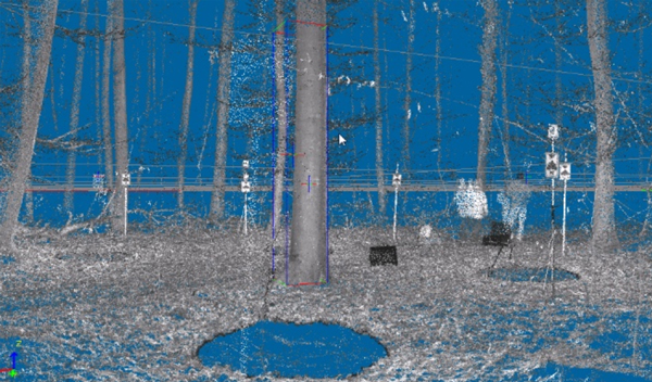
Fig. 1. Scan output showing a targeted beech. This scan was performed from four different directions.
For scanning, the Zoller+Fröhlich Imager 5006 was used, this scanner is built around the phase shift principle. A disadvantage of this principle is that distances larger than 79 m cannot be assessed. However, as the scanner was positioned at a distance to the tree between 2.7 m and 17.3 m, this problem did not occur. The larger distance was used in cases of combined scanning of two adjacent trees in a hilly terrain abundantly covered with vegetation. The trees were scanned in “super high resolution”, i.e. 20 000 pixels per 360° in horizontal and vertical directions. As the pixel resolution of the scanned point cloud is 3.1 mm for a distance of 10 m in this modus, the resolution is 2.4 mm for the arithmetic mean for the distances of the trees to the scanner (7.8 m).
After felling the trees they were cut to log lengths with a length of approximately 4 m each. The logs were numbered starting with number one on the tree length up to approximately 4 m, following by number 2 and if necessary by number 3. For this first test, we only used the first and second parts of the trees U, V, W and Y, i.e. U1, U2, V1, V2, W1, W2, Y1, and Y2. Each bark characteristic was numbered according to the tree number and part. Additionally all visible bark scars and similar characteristics were measured manually post harvest. The position was measured by a measuring tape (accuracy 1 mm) in relation to a reference line along the log beginning at one log end. The two coordinates were the length along the line and the distance to the line. Then the width and length of all characteristics were measured by the measuring tape. Fig. 2 shows the four different parameters which were also measured by use of the TLS data: Scar width and height and width and height of the branched knot.
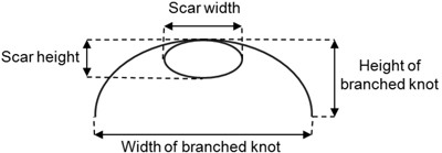
Fig. 2. Parameters measured at each bark characteristic.
3 Methods
3.1 3D reconstruction of the tree stem surface
As a first step of this new approach the raw data of each tree needs to be processed. All scans per tree are oriented to each other by the Zoller+Fröhlich LaserControl software, with an average accuracy of 1.0 mm. The result is one Cartesian coordinate system to describe the location of all scanned points. The points of each scan belonging to the surface of a tree stem are isolated using the filter functions of the Zoller+Fröhlich LaserControl software. Points are then merged to a file consisting of points which represent the actual surface of the tree stem. This file is then processed by our own software using the algorithms presented by Pfeifer et al. (2004b) to build a chain of cylinders along the tree axis. The result is a text file with the coordinates denoting the center of each cylinder, the cylinder axis as a 3D vector, and the radius.
3.2 Introduction of an additional coordinate system
In Fig. 3 the centers of two cylinders are connected to build up a local coordinate system with the conventional axes x, y, and z (red).
To distinguish small differences on the stem surface within the laser scan data, an alternative coordinate system is introduced: Cartesian coordinates {x,y,z} are replaced by a new set of variables {L,z,d}, where L is the arc length, d is the distance to the nearest point of the cylinder surface, and z the height on the tree stem (see Fig. 3). According to Bronstein and Semendjajew (1985) the resulting coordinate system is referred to as a cylindrical coordinate system. Compared to the spherical or polar coordinate system the parameter d is measured on a plane rectangular to the cylinder axis in contrast to the distance of this point to the origin of the coordinate system as being true for a spherical or polar coordinate system.
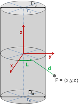
Fig. 3. New coordinate system {L,z,d} with cylinders as a basis to evaluate height differences with respect to the bark surface. Each point P of the laser scanning image can be defined in 3D space either in a Cartesian coordinate system by {x,y,z} or by the set {L,z,d} linked to the virtual cylinders describing a simplified tree stem surface. The axis of the cylinder is given by a pair of points ru and rd. Diameters of the top and bottom areas of the cylinder are denoted as Du and Dd.
3.3 Coordinate transformation
The visualized part of the tree stem is characterized by two points (ru = {xu,yu,zu} and rd = {xd,yd,zd}) and diameters of the area of the top and bottom (Du and Dd ), respectively (see Fig. 3). The actual position of each point of the cloud in Cartesian coordinates P = {x,y,z} is also known. The distance d between the point P and an approximated stem shape as well as the arc length L at the same height z specifies the shape function of the actual tree surface.
The values L and d are calculated from coordinates x, y, and z by use of the parameters ru, rd, Du, and Dd. Fig. 4 illustrates the distance between the point P = {x,y,z} and cylinder axis rp = {xp,yp,zp} in the same z-plane z = zp.
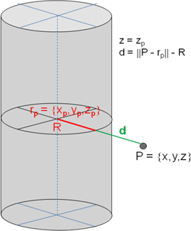
Fig. 4. Illustration of parameter d as the distance from the cylinder surface to point P.
Parameter d is captured by Eq. 1.
![]()
Parameter d is captured by Eq. 1, where R is the virtual cylinder radius calculated as follows (Eq. 2):

The parametric form of the line equation connecting points ru and rd allows to link two unknown variables xp, and yp with the known ones.

![]()
![]()
Substitution of xp, yp and R from Eq. 1 with those in Eq. 2 and Eq. 3 to Eq. 5 provides the value for variable d.
Arc length L corresponding to point P = {x,y,z} is shown in Fig. 5.
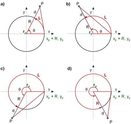
Fig. 5. Arc length L dependent on the position of P in the x-y coordinate system.
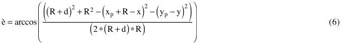
Here, the law of cosines for the triangle with vertices {{x,y},{xp,yp},{xp + R,yp}} in plane z = zp is applied to provide a mathematical framework for the calculation of the central angle θ (see Eq. 6) and the circular arc L (see Eq. 7 and Eq. 8).
![]()
![]()
3.4 Visualization
In Fig. 6 a tree bark area of specific interest is visualized utilizing the conventional {x,y,z} coordinate system. The graphics were made by use of the corresponding functions of the numerical computing environment MATLAB developed by MathWorks (version R2011b and R2013a).
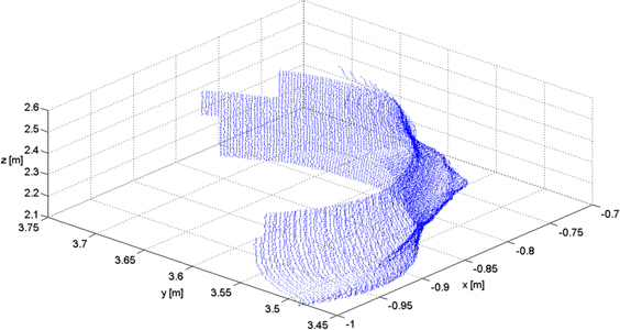
Fig. 6. The point cloud characterizing the user defined bark feature in 3D modus of the laser scanning image (conventional x,y,z system).
Fig. 7 shows the point cloud transformed to the {L,z,d} coordinate system. Here, the corresponding surface is projected onto a plane without stretching, tearing or shrinking. The basis of this coordinate system is the stem of the tree represented by a chain of cylinders.
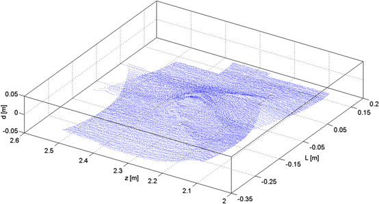
Fig. 7. Transformed 3D point cloud in the L,z,d coordinate system.
To enable precise and accurate measurements of the surface feature as a shape and not as a collection of single points, meshing is required. Thus, the scattered data set defined by locations {L,z} and corresponding values d is interpolated using a Delaunay triangulation (de Berg et al. 2008) of {L,z}. Function F for the calculation of the interpolation is assessed using the TriScatteredInterp class provided by MATLAB.
Following our new approach, Fig. 8 shows the 3D surface of the interpolated point cloud. Distance parameter d is linked with the jet color map provided by MATLAB in our application. This color map begins with blue, and passes through cyan, yellow, orange, and red. Thus, the points with minimal d values are shown in blue, those with maximum values of d in red. This coloring technique visualizes small changes in the geometric shape of the bark characteristics. By use of the two-norm of a vector connecting two points of this surface, the distance between them along the side of the virtual cylinder representing the tree stem can be calculated. The distance measurements are similar to the manual measurements of the bark characteristics of the real tree. Similar features observable on the bark on the tree are visualized and therefore measurable with our method in case the edges show small differences on the stem surface. Thus, this approach allows the measurement of tree bark features with a precision of 1 mm.
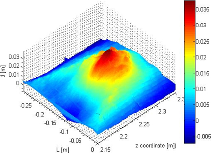
Fig. 8. The surface of a portion of a stem obtained by interpolation of the 3D point cloud is shown from an arbitrary point of view. The lower regions denoted in blue are below or even with the approximated stem surface. Yellow and red represent regions considerably higher than the surface of the stem approximated by cylinders.
We also investigated other options for the reconstruction of tree bark by creating contour lines together with the 3D surface and further analysis of their projection to the {L,z}- plane. Each isoline of the 2D contour plot representing the 3D tree stem surface connects points of equal distance parameter d above a given level defined by the surface of the virtual cylinder. Fig. 9 presents an example for the numerical simulation of the bark surface projected into the {L,z}- plane for one of the beech trees.
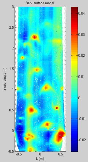
Fig. 9. Numerical reconstruction of the tree stem surface. By applying a coordinate transformation the stem of a tree is projected into a new coordinate system with z as the height above or below the scanner axis and L as the distance around the stem rectangular to the z-axis. The third dimension, the distance above or below the approximated cylinder surface, i.e. distance parameter d, is represented by colors ranging from blue (below or even with the cylinder surface) to red (points high above the cylinder surface).
The visualized stem section shows the distance parameter d of the laser scanner from z = -0.5 m to 3 m. The complete length of this tree up to the crown of 5.7 m is covered by a chain of 55 virtual cylinders, each directed along the tree stem axis within the same z-interval. The horizontal lines are related to the boundary between a pair of neighboring cylinders. Specific bark features on the tree stem surface can visually be detected due to the chosen jet-color map: Scars and branched knots are shown in green-yellow-red spectrum.
4 Results
As a first approach we detected and measured 18 bark scars in the TLS data of three trees (denoted V, W, and Y). One tree was omitted from further evaluation as the scans did not return sufficient quality due to the steep terrain. The first results show that not all scars could be detected using this new 3D approach, as not all of them show a distinguishable deviation from the cylinder surface. In these cases such scars are measured by use of intensity data as proposed by Schütt et al. (2004). Table 1 shows the measurement results of these 18 scars.
| Table 1. Comparison of scars and branched knots measured manually and by use of TLS data. The trees taken into account were denoted V, W, and Y. As the logs were cut in parts, they were numbered V1, V2, W1, W2, Y1, and Y2. Each characteristic measured manually was then numbered beginning with the first measurement. The name of the characteristic indicates the log part it was found on, e.g. V1_1 means first characteristic on the first log of tree V. | ||||||||
| Scar number | Scar width [cm] | Scar height [cm] | Width of branched knot [cm] | Height of branched knot [cm] | ||||
| Manually | By TLS data | Manually | By TLS data | Manually | By TLS data | Manually | By TLS data | |
| V1_1 | 8.4 | 2.34 a) | 2.0 | 2.87 a) | 37.0 | 35.40 a) | 2.2 | 2.75 a) |
| V1_7 | 9.9 | 6.18 a) | 3.8 | 3.06 a) | 37.5 | 25.66 a) | 8.0 | 4.68 a) |
| V1_15 | 8.3 | 6.89 a) | 2.2 | 2.01 a) | 27.0 | 26.62 a) | 2.2 | 2.01 a) |
| V2_2 | 10.0 c) | 10.80 a) | 3.1 | 3.53 a) | --- | --- | 3.1 | --- |
| V2_6 | 12.0 | 7.15 b) | 11.0 | 12.47 b) | 57.0 | 16.26 b) | 16.0 | 21.34 b) |
| V2_12 | 6.7 | 8.05 a) | 4.8 | 4.64 a) | 34.2 | 30.70 a) | 8.7 | 7.03 a) |
| W1_3 | 13.5 | 13.44 b) | 4.0 | 3.74 b) | 37.5 | 38.54 b) | 6.5 | 4.67 b) |
| W1_6 | 6.2 | 4.03 b) | 2.0 | 1.58 b) | 25.0 | 21.29 b) | 3.0 | 3.52 b) |
| W1_10 | 4.0 | 4.14 a) | 2.8 | 2.92 a) | 19.0 | 7.79 a) | 7.0 | 5.65 a) |
| W2_11 | 5.4 | 5.58 a) | 6.2 | 6.18 a) | 36.0 | 13.82 a) | 18.8 | 11.35 a) |
| W2_15 | 4.5 | 4.45 a) | 5.0 | 5.82 a) | 27.0 | 17.30 a) | 21.0 | 14.80 a) |
| W2_16 | 6.0 | 5.15 a) | 6.2 | 5.91 a) | 28.0 | 22.20 a) | 18.0 | 16.60 a) |
| Y1_1 | 6.0 | 6.47 a) | 2.3 | 3.15 a) | 17.0 | 15.20 a) | 3.7 | 4.10 a) |
| Y1_2 | 10.5 | 12.68 a) | 3.7 | 4.23 a) | 40.5 | 34.20 a) | 6.8 | 6.20 a) |
| Y1_3 | 14.5 | 11.11 a) | 2.7 | 2.36 a) | 30.0 | 26.44 a) | 5.0 | 2.36 a) |
| Y2_3 | 9.6 | 7.57 a) | 3.5 | 3.91 a) | 27.0 | 29.90 a) | 4.9 | 4.90 a) |
| Y2_23 | 18.2 | 11.14 b) | 4.2 | 5.06 b) | 43.0 | 43.22 b) | 8.5 | 10.34 b) |
| Y2_27 | 14.3 | 10.48 b) | 8.3 | 8.17 b) | 35.0 | 36.33 b) | 14.0 | 11.88 b) |
| a) TLS measurements were performed by intensity data. b) TLS measurements were performed by use of the bark surface model. c) This result is not reliable due to the geometry of the intensity data. | ||||||||
To get a first impression of our technique, differences were calculated by subtracting the measurement result by TLS data from those values derived manually (Table 2).
| Table 2. Differences between the manual measurements on the felled tree and the measurements of the scars and branched knots by use of TLS data. The trees taken into account were denoted V, W, and Y. As the logs were cut in parts, they were numbered V1, V2, W1, W2, Y1, and Y2. Each characteristic measured manually was then numbered beginning with the first measurement. The name of the characteristic indicates the log part it was found on, e.g. V1_1 means first characteristic on the first log of tree V. | ||||||||
| Scar number | Scar width | Scar height | Width of branched knot | Height of branched knot | ||||
| Manual meas. [cm] | Difference [cm] | Manual meas. [cm] | Difference [cm] | Manual meas. [cm] | Difference [cm] | Manual meas. [cm] | Difference [cm] | |
| V1_1 | 8.4 | 6.06 | 2.0 | –0.87 | 37.0 | 1.60 | 2.2 | –0.55 |
| V1_7 | 9.9 | 3.72 | 3.8 | 0.74 | 37.5 | 11.84 | 8.0 | 3.32 |
| V1_15 | 8.3 | 1.41 | 2.2 | 0.19 | 27.0 | 0.38 | 2.2 | 0.19 |
| V2_2 | 10.0 | –0.80 | 3.1 | –0.43 | 0.00 | 3.1 | 3.10 | |
| V2_6 | 12.0 | 4.85 | 11.0 | –1.47 | 57.0 | 40.74 | 16.0 | –5.34 |
| V2_12 | 6.7 | –1.35 | 4.8 | 0.16 | 34.2 | 3.50 | 8.7 | 1.67 |
| W1_3 | 13.5 | 0.06 | 4.0 | 0.26 | 37.5 | –1.04 | 6.5 | 1.83 |
| W1_6 | 6.2 | 2.17 | 2.0 | 0.42 | 25.0 | 3.71 | 3.0 | –0.52 |
| W1_10 | 4.0 | –0.14 | 2.8 | –0.12 | 19.0 | 11.21 | 7.0 | 1.35 |
| W2_11 | 5.4 | –0.18 | 6.2 | 0.02 | 36.0 | 22.18 | 18.8 | 7.45 |
| W2_15 | 4.5 | 0.05 | 5.0 | –0.82 | 27.0 | 9.70 | 21.0 | 6.20 |
| W2_16 | 6.0 | 0.85 | 6.2 | 0.29 | 28.0 | 5.80 | 18.0 | 1.40 |
| Y1_1 | 6.0 | –0.47 | 2.3 | –0.85 | 17.0 | 1.80 | 3.7 | –0.40 |
| Y1_2 | 10.5 | –2.18 | 3.7 | –0.53 | 40.5 | 6.30 | 6.8 | 0.60 |
| Y1_3 | 14.5 | 3.39 | 2.7 | 0.34 | 30.0 | 3.56 | 5.0 | 2.64 |
| Y2_3 | 9.6 | 2.03 | 3.5 | –0.41 | 27.0 | –2.90 | 4.9 | 0.00 |
| Y2_23 | 18.2 | 7.06 | 4.2 | –0.86 | 43.0 | –0.22 | 8.5 | –1.84 |
| Y2_27 | 14.3 | 3.82 | 8.3 | 0.13 | 35.0 | –1.33 | 14.0 | 2.12 |
No widths or heights were larger than 57.0 cm. Therefore, we assume that differences exceeding 5.0 cm on the scars or branched knots should be rated as false identifications. This can be considered true for 12 results. Seven of which occur when measuring the width of branched knots. The reason for this problem may be that branched knots often have no severe distance parameter d or intensity modifications in the outbound areas.
Examining the remainder of the differences it can be distinguished that 31% of the differences are negative. The reason may be the similar as above, the edges of such surface features are often poorly recognizable with little change in relief. Excluding the 12 values with differences exceeding 5.0 cm, the remaining values vary from 0.0 cm to 4.85 cm, 1.1 cm being the arithmetic mean.
5 Discussion
Our approach to measure scars and branched knots by use of TLS data leads to difficulties when the characteristic parameters are not evident or of an insufficient quality to identify. In such cases the differences between TLS data and manual measurements are too large to count the result as a measurement. This is true for differences which exceed 5.0 cm, and must be excluded from further analysis. In cases where the contrast to adjacent regions where height or intensity information is sufficient, scars are not only well recognizable but also the results for scar height measurement are accurate to within 1.0 cm (58% of the results measured by TLS data show a difference below 1.0 cm). This shows that for specific stem surface characteristics this method may be the basis of a solution for the quality assessment of standing trees.
As the manual measurements were applied to all characteristics observed on the tree stem, all features identified by our approach could be related to these measurements. As focus of this approach is on scars and branched knots, these were selected manually from the TLS data. Artificially pruned branches are especially easy to detect by this approach. In this first development we concentrated on the treatment of beech trees. A transfer of this approach to species with a significantly different bark structure may be a challenge.
In contrast to Thomas and Thomas (2011) we have not yet implemented a fully automated detection system, but the mathematic methodology may serve as a basis to do so. Thomas and Thomas (2011) have reached a multi-purpose solution whereas this study only focuses on a specific characteristic. The minimal distance above the approximated cylinder of our characteristics identified so far is 1.2 cm. This is more or less the same as 0.5 inches (1.3 cm), comparable with the work by Thomas and Thomas (2011). Their approach is employed within sawmills post felling of the tree, whereas we offer a solution for standing in-situ trees.
The resolution of the data after mapping it on a surface is the main drawback of the approach of Schütt et al. (2004). The shape of the characteristic is difficult to detect as he uses intensity data. Our approach was to additionally use a bark surface model which offers easy localization of characteristics which have a distinguished distance parameter d in contrast to the surroundings. Then, highly accurate measurements are feasible. Our results are comparable with the manual measurement of scars on a felled tree.
6 Conclusion and outlook
In this paper, we presented first results of our approach to measure bark scars and branched knots of beech trees by use of TLS data. In cases where an alternative to the measurement of intensity data was required, the bark points were transformed into a cylindrical coordinate system to establish a bark surface model. Here, the distance parameter d of stem points above a reference cylinder is the main attribute for further investigation of the stem.
In a further step we plan to analyze further measurements to identify the limitations of the approach by the use of intensity data as well as the bark surface model. Then, bark scars which are higher (more pronounced) than the identified threshold can be automatically detected. Such a methodology can be used to automatically determine the quality category of a tree stem. Moreover, the shape of the scars can also be automatically detected by use of isolines. This offers an objective method to measure scars on the tree bark in contrast to manual measurements, the precision of which depend highly on the skill of the measurement taker. To do so, all isolines above a certain threshold are separated. As an example of this approach isolines are shown as solid black lines in Fig. 10.
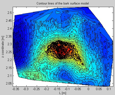
Fig. 10. Assembly of contour lines above a user-defined threshold. These lines are indicated by solid black lines.
In a first step this threshold is defined by the user. The assembly of lines allows for the targeted extraction of the sample set {L,z,d} of each single bark characteristic and to provide an approximation of the shape using a curve. As a first approach we use a Gaussian approximation as well as Fourier Models (see Fig. 11 and Fig. 12).
The main shape of the characteristic is best captured by an approximation with a small degree. The best fit can be accomplished by using a Fourier approximation of degree 2 within the borders of the characteristic (see the green line in Fig. 12).
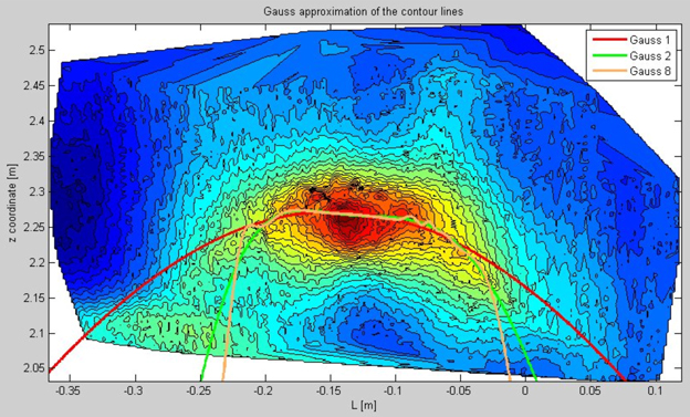
Fig. 11. Gaussian approximation of a bark characteristic with modifying degrees (1 = red, 2 = green, 8 = brown).
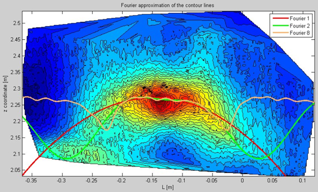
Fig. 12. Fourier approximation of a bark characteristic with modifying degrees (1 = red, 2 = green, 8 = brown).
Acknowledgements
The FlexWood project (www.flexwood-eu.org) was funded by the European Union within the Seventh Framework Programme (FP7). The Collaborative Project (small or medium sized focused research project) contributes to “Meeting industrial requirements on wood raw-materials quality and quantity” activities [FP7 Grant Agreement No. 245136]. We would especially like to thank the team lead by Franka Brüchert at the Forest Research Institute Baden-Württemberg, a FlexWood project partner, for the provision of manual measurement data that was used within this article.
References
Aschoff T., Thies M., Spiecker H. (2004). Describing forest stands using terrestrial laser-scanning. In: Altan M.O. (ed.). Geoimagery bridging continents. Proceedings and results of XXth ISPRS Congress, Istanbul, Turkey. International Archives of Photogrammetry, Remote Sensing, and Spatial Information Sciences XXXV: 237–241.
Bienert A., Scheller S. (2008). Verfahren zur automatischen Bestimmung von Forstinventurparametern aus terrestrischen Laserscannerpunktwolken. In: Seyfert E. (ed.). DGPF Tagungsband 2008 – Vom Erdapfel zum 3D-Modell. Publikationen der Deutschen Gesellschaft für Photogrammetrie, Fernerkundung und Geoinformation e.V. 17: 37–46.
Bronstein I.N., Semendjajew K.A. (1985). Taschenbuch der Mathematik. BSB B.G. Teubner Verlagsgesellschaft, Leipzig.
De Berg M., Cheong O., van Kreveld M., Overmars M. (2008). Computational geometry. Algorithms and Applications. Third edition. Springer.
Hopkinson C., Chasmer L., Young-Pow C., Treitz P. (2004). Assessing forest metrics with a ground-based scanning lidar. Canadian Journal of Forest Research 34: 573–583. http://dx.doi.org/10.1139/x03-225.
Liang X., Litkey P., Hyyppa J., Kukko A., Kaartinen H., Holopainen M. (2008). Plot-level trunk detection and reconstruction using one-scan-mode terrestrial laser scanning data. In: Weng Q., Zhang J. (eds.). Proceedings of the International Workshop on Earth Observation and Remote Sensing Applications (EORSA) 2008. p. 1–5.
Liang X., Kankare V., Yu X., Hyyppä J., Holopainen M. (2014). Automated stem curve measurement using terrestrial laser scanning. IEEE Transactions on Geoscience and Remote Sensing 52(3). http://dx.doi.org/10.1109/TGRS.2013.2253783.
Litkey P., Liang X., Kaartinen H., Hyyppä J., Kukko A., Holopainen M. (2008). Single-scan TLS methods for forest parameter retrieval. In: Hill R.A., Rosette J., Suárez J. (eds.). Proceedings of SilviLaser 2008: 8th international conference on LiDAR applications in forest assessment and inventory, Edinburgh, UK. p. 295–304.
Pal I. (2008). Measurements of forest inventory parameters on terrestrial laser scanning data using digital geometry and topology. In: Chen J. (ed.). Silk road for information from imagery. Proceedings and results of the XXIst ISPRS Congress, Beijing, China. The International Archives of the Photogrammetry, Remote Sensing and Spatial Information Sciences XXXVII: 373–380.
Pfeifer N., Gorte B., Winterhalder D. (2004a). Automatic reconstruction of single trees from terrestrial laser scan data. In: Altan M.O. (ed.). Geo-imagery bridging continents. Conference proceedings ISPRS conference in Istanbul, Istanbul, Turkey. International Archives of Photogrammetry, Remote Sensing, and Spatial Information Sciences XXXV.
Pfeifer N., Winterhalder D. (2004b). Modelling of tree cross sections from terrestrial laser-scanning data with free-form curves. In: Thies M., Koch B., Spiecker H., Weinacker H. (eds.). Laser-scanners for forest and landscape assessment. Proceedings of the ISPRS working group VIII/2, Freiburg, Germany. International Archives of Photogrammetry, Remote Sensing, and Spatial Information Sciences XXXVI: 76–81.
Schütt C., Aschoff T., Winterhalder D., Thies M., Kretschmer U., Spiecker H. (2004). Approaches for recognition of wood quality of standing trees based on terrestrial laserscanner data. In: Thies M., Koch B., Spiecker H., Weinacker H. (eds.). Laser-scanners for forest and landscape assessment. Proceedings of the ISPRS working group VIII/2, Freiburg, Germany. International Archives of Photogrammetry, Remote Sensing, and Spatial Information Sciences XXXVI: 179–182.
Simonse M., Aschoff T., Spiecker H., Thies M. (2003). Automatic determination of forest inventory parameters using terrestrial laser scanning. In: Hyyppä J., Næsset E., Olsson H., Granqvist Pahlén T., Reese H. (eds.). Proceedings of the ScandLaser Scientific Workshop on Airborne Laser Scanning of Forests, Umeå, Sweden. p. 252–258.
Thomas L., Thomas R.E. (2011). A graphical automated detection system to locate hardwood log surface defects using high-resolution three-dimensional laser scan data. In: Fei S., Lhotka J.M., Stringer J.W., Gottschalk K.W., Miller G.W. (eds.). Proceedings, 17th Central Hardwood Forest Conference, Newtown Square, PA, USA. U.S. Department of Agriculture, Forest Service, Northern Research Station, General Technical Report NRS-P-78: 92–101.
van Goethem G.R.M., van de Kuilen J.W.G., Gard W., Ursem W.N.J. (2008). Quality assessment of standing trees using 3D laserscanning. In: Gard W., van de Kuilen J.W.G. (eds.). COST E53 Conference Proceedings – end user’s needs for wood material and products. p. 145–156.
Watt P.J., Donoghue D.N.M. (2005). Measuring forest structure with terrestrial laser scanning. International Journal of Remote Sensing 26: 1437–1446. http://dx.doi.org/10.1080/01431160512331337961.
Total of 16 references
