Rami Saad  ,
Jörgen Wallerman,
Johan Holmgren,
Tomas Lämås
,
Jörgen Wallerman,
Johan Holmgren,
Tomas Lämås
Local pivotal method sampling design combined with micro stands utilizing airborne laser scanning data in a long term forest management planning setting
Saad R., Wallerman J., Holmgren J., Lämås T. (2016). Local pivotal method sampling design combined with micro stands utilizing airborne laser scanning data in a long term forest management planning setting. Silva Fennica vol. 50 no. 2 article id 1414. https://doi.org/10.14214/sf.1414
Highlights
- Most similar neighbor imputation was used to estimate forest variables using airborne laser scanning data as auxiliary data
- For selecting field reference plots the local pivotal method (LPM) was compared to systematic sampling design
- The LPM sampling design combined with a micro stand approach showed potential for improvement and has the potential to be a competitive method when considering cost efficiency.
Abstract
A new sampling design, the local pivotal method (LPM), was combined with the micro stand approach and compared with the traditional systematic sampling design for estimation of forest stand variables. The LPM uses the distance between units in an auxiliary space – in this case airborne laser scanning (ALS) data – to obtain a well-spread sample. Two sets of reference plots were acquired by the two sampling designs and used for imputing data to evaluation plots. The first set of reference plots, acquired by LPM, made up four imputation alternatives (varying number of reference plots) and the second set of reference plots, acquired by systematic sampling design, made up two alternatives (varying plot radius). The forest variables in these alternatives were estimated using the nonparametric method of most similar neighbor imputation, with the ALS data used as auxiliary data. The relative root mean square error (RelRMSE), stem diameter distribution error index and suboptimal loss were calculated for each alternative, but the results showed that neither sampling design, i.e. LPM vs. systematic, offered clear advantages over the other. It is likely that the obtained results were a consequence of the small evaluation dataset used in the study (n = 30). Nevertheless, the LPM sampling design combined with the micro stand approach showed potential for improvement and might be a competitive method when considering the cost efficiency.
Keywords
LIDAR;
forest management planning;
local pivotal method (LPM);
segmentation;
most similar neighbor (MSN) imputation;
suboptimal loss;
Heureka;
decision support system
-
Saad,
Swedish University of Agricultural Sciences (SLU), Department of Forest Resource Management, Skogsmarksgränd, SE-901 83 Umeå, Sweden
E-mail
rami.saad@slu.se
- Wallerman, Swedish University of Agricultural Sciences (SLU), Department of Forest Resource Management, Skogsmarksgränd, SE-901 83 Umeå, Sweden E-mail jorgen.wallerman@slu.se
- Holmgren, Swedish University of Agricultural Sciences (SLU), Department of Forest Resource Management, Skogsmarksgränd, SE-901 83 Umeå, Sweden E-mail johan.holmgren@slu.se
- Lämås, Swedish University of Agricultural Sciences (SLU), Department of Forest Resource Management, Skogsmarksgränd, SE-901 83 Umeå, Sweden E-mail tomas.lamas@slu.se
Received 29 June 2015 Accepted 10 December 2015 Published 26 January 2016
Views 82088
Available at https://doi.org/10.14214/sf.1414 | Download PDF

1 Introduction
In forest management and planning, the notion stand is used as both a description and treatment unit for a piece of (in several aspects) homogenous forest land. A single treatment (silvicultural or harvest actions) is assumed to be applied on the whole stand at a single point of time and stands thereby makes up the basic unit in forest planning (e.g., Bettinger et al. 2009). Decision support systems (DSSs), such as the Swedish Heureka system (Wikström et al. 2011), can be used to simulate and evaluate different possible standwise treatments for each stand separately or jointly for all stands within a forest holding. Recent studies (Pietilä et al. 2010; Saad et al. 2014) have attempted to test different data acquisition methods where the treatment units, i.e., stands, are based on the traditional conception of forest stands. Stand variation in size and shape can be an important factor affecting the data quality of the variables of interest. Highly accurate data regarding forest information are critical for analyzing potential management actions in forest planning (Kangas 2010). Inaccurate forest data can lead to a decrease in economic gain due to subsequent erroneous treatment decisions (Holmström et al. 2003). Despite the importance of data quality in forest planning, the subject has not received much attention compared to other aspects of forest planning and data acquisition (Duvemo and Lämås 2006). Kangas (2010) has emphasized the complexity of the subject and suggested methods, such as the Bayesian decision theory, to improve the use of the available forest data.
Stand delineation is an important procedure aimed at reducing variety within the delineation units by uniting similar forest areas, such as those with similar tree species, tree height, development class or site index. Historically, forests have been delineated manually, either by field survey or aerial photo interpretation. Since stand delineation is performed manually and subjectively, a high variation in forest characteristics within stands is often encountered. Nowadays, stand delineation can be performed with different automatic segmentation algorithms using remote sensing (Olla 1990; Hyvönen et al. 2005). The use of airborne laser scanning (ALS) data in such procedures (Koch et al. 2009) can potentially reduce within stand variation of forest characteristics, thereby improving stand data quality. Such an automatic segmentation method was recently developed by Olofsson and Holmgren (2014), in order to reduce within stand variation according to the ALS derived variables. The use of ALS data and automatic stand delineation have enabled the introduction of very small forest stands, known as micro stands (Hyvönen et al. 2005; Pippuri et al. 2012), as a potentially improved way to divide a forest into homogeneous areas for use as the description unit in management planning. Whereas traditional stands (in Sweden) might range between 1–10 ha, micro stands are typically the size of 0.1 ha. In management planning process micro stands can be aggregated to treatment units.
Using the micro stand approach, the forest state in each micro stand has to be estimated. If using the combination of remote sensing and field survey the challenge is then to allocate field reference plots in an efficient manner. Field plots can be allocated in a systematic grid within the forest area but also, e.g., the location of plots within a stratified sample of (traditional) stands. Using micro stands field plots can be allocated in a – somehow selected – sample of micro stands.
Selecting the units to be sampled is a general problem in sampling. A new sampling method called the local pivotal method (LPM) was proposed by Grafström et al. (2012). LPM provides a well-spread sample compared to, e.g., systematic and simple random sampling designs when data such as ALS data can be used as auxiliary variables. The LPM uses the distance between units in an auxiliary space to achieve a spatially balanced sample. In the present study, the LPM approach was utilized by employing ALS data as the auxiliary variables to achieve a well-spread sample in the auxiliary space.
For estimating stand attributes for each micro stand imputation technique such as the nonparametric most similar neighbor (MSN) method (Moeur and Stage 1995) utilizing ALS as auxiliary data and field reference plots is a potential method (Packalén and Maltamo 2007; Maltamo at al. 2009). Using this approach, no parametric assumptions are made regarding, e.g., the relationship between stand attributes and ALS data.
The accuracy of data acquired from combining remote sensing and field surveys depends on several factors, such as the characteristics of the data from the two sources, respectively, and the method used for combining them. For cost efficiency fast field surveys are advantageous and combining the micro stand and LPM approaches may provide a faster field survey design compared to other sampling designs. However the time consumption for different field survey designs was not the scope in this study.
The aim of the study was to test the efficiency of (i) the new sample design, LPM, combined with micro stand approach and then compare it with a (ii) traditional layout of reference plots in a systematic grid over the forest area. In both cases (i and ii) the forest variables were estimated using the MSN imputation method by employing ALS data as auxiliary information. In (i), the allocation of reference plots among the selected micro stands and geographical location of plots within the micro stands were carried out using the recently developed LPM, using ALS data as auxiliary information. Another aim was to investigate the effect of these approaches on long term forest planning (100 years) in terms of suboptimal losses in management decisions.
2 Material and methods
2.1 Study area and data
This study was performed using data obtained from the Remningstorp estate located in southern Sweden (58°30´N, 13°40´E). This forest holding covers about 1200 ha of productive forest land and the forests within the holding have frequently been used for remote sensing research projects. The prevailing tree species are Norway spruce (Picea abies (L.) H. Karst.), Scots pine (Pinus sylvestris L.) and birch (Betula spp.). The dominant soil type is till (i.e., mixture of glacial debris) with a field layer consisting of different herbs, blueberry (Vaccinium myrtillus L.) and narrow leaved grass (e.g., Deschampsia flexuosa (L.) Trin.). However, in the dense old spruce stands, the field layer is in general absent. The ground elevation varies moderately from 120 m to 145 m above sea level. The Remningstorp estate is managed for commercial wood production by “The Swedish Forest Society Foundation” (Skogssällskapet) and the forest includes development states from young to old forest.
ALS data acquisition was performed by scanning from a helicopter on 29 August and 9 September 2010 with a Riegl LMS-Q560 system. The area was scanned from a flight height of approx. 400 m above ground level and the pulse density was at least 10 measurements per square meter. The laser wavelength was 1550 nm and the beam divergence was 0.5 mrad. A parallel scan pattern was used and the maximum scan angle was ±30 degrees from nadir across the flight direction.
The vertical distance to the ground was calculated for each laser return using a ground elevation model and laser metrics were derived twice based on the distribution of these heights within each two different raster cell sizes, 10 × 10 m2 and 18 × 18 m2. The metrics were as follows: (1) average height (AH), (2) standard deviation of heights (SDH), (3) vegetation ratio (VR), (4), average crown height (ACH), (5) 10th height percentile (P10), (6) 50th height percentile (P50), and (7) 90th percentile (P90). The metrics AH, SDH and the percentiles were derived based only on the laser returns that were above a height threshold of 2 m in order to avoid any influence from low vegetation, stones, etc. The metric used to describe the vegetation density (VR) was calculated by dividing the number of returns above a threshold of 2 m from the ground by the total number of returns. The metric for measuring both the canopy height and crown closure, i.e., the average crown height (ACH), was calculated from a canopy height model (CHM). First, a 3 × 3 m2 median filter was applied on the CHM with a raster cell size of 1 × 1 m2 to fill in missing values. To derive the ACH for a 10 × 10 m2 and 18 × 18 m2 raster cells, the average height value of all raster cells of the CHM inside the 10 × 10 m2 raster cell was calculated.
Data obtained using the LPM sampling design (5 m radius plots) and systematic sampling design (10 m radius plots) were used as reference data (training data) in different subsets and combinations to predict the forest state from the ALS data. Data from 40 m radius plots were used to evaluate the predictions as these data were similar in size and characteristics to micro stands and were available for a wide range of forest types.
2.1.1 Systematic sampling design
The systematic sample included 10 m radius plots surveyed in 2010 and located in a 200 × 200 m grid over the major part of the estate, resulting in 263 plots located on forest land. This data set was available prior to the present study and used in several other remote sensing research projects. The plots were surveyed using the methods and models estimating the state of the forest available in the Heureka system by employing the modules Ivent and PlanStart (Wikström et al. 2011). For plots with a mean tree height less than 4 m or basal-area-weighted mean stem diameter at breast height (i.e., 1.3 m above ground) less than 5 cm, only the height and species of all saplings and trees were recorded. For the remaining plots, calipering of all trees greater than 4 cm in diameter at breast height and sub-sampling of trees to measure height and age were performed. Heights of the remaining calipered trees on the plots were estimated using allometric models relating tree height to diameter (Söderberg 1992). Only plots with calipered trees were used, i.e., young forest was not included. Furthermore, to eliminate errors due to silvicultural activities performed or disturbances due to, e.g., wind throw between the time of field survey and ALS scanning, plots showing extreme deviation from the expected relationship to the ALS measurements were removed. In total, 216 plots were used. Table 1 provides a summary of the data collected.
| Table 1. Summary statistics of the datasets (min; mean; max). | |||||
| Dataset | Number of plots | Tree height [m] | Stem diameter [cm] | Stem volume [m3/ha] | Age [yr] |
| Micro stand and LPM approach | 856* | 3.5;19.2;34 | 4;27.1;67.9 | 1;284;2058 | 10;50;168 |
| Systematic design | 216** | 4.9;18.2;31.6 | 5.2;24.1;51.9 | 2;229;655 | 14;51;160 |
| Evaluation plots | 30*** | 15.8;24;32.4 | 20;30.6;42.3 | 157;360;685 | 33;60;112 |
| * 5 m radius ** 10 m radius *** 40 m radius LPM = local pivotal method | |||||
2.1.2 LPM sampling design
For the LPM sampling design, the forest area was first delineated into micro stands based on ALS data using the segmentation algorithm developed by Olofsson and Holmgren (2014) and raster cells of 10 × 10 m2 as input. The input raster contained three bands with ALS metrics: P90, VR and ACH. Non-forest areas and roads were excluded from the segmentation using a raster mask. The raster mask was generated using both the spatial database earlier used for forest management and road vectors identified from aerial images. Next, 5 m radius plots were allocated to a sub-sample of 100 micro stands selected using the LPM (Grafström et al. 2012). Each of these micro stands was visited, but nine micro stands were not surveyed or included in the study because of thinning operations after the ALS data acquisition. Therefore, 91 micro stands in total were surveyed in 2013 and used in this study. The LPM sampling design has been proven to select a well-spread sample in a given space (Grafström et al. 2012), i.e., it is unlikely that two similar (in ALS space) micro stands will be selected in the sample. In this study, the LPM was applied using the standardized ALS metrics AH, SDH, VR, ACH, P10, P50, and P90 for measuring the distance between units, i.e., the selected micro stands were spread in the auxiliary data (ALS metrics) space. The probability of selecting a particular micro stand was set proportionally to the sum of ACH for all raster cells within the micro stand because this sum was correlated to the total stem volume. The reason for this selection was to ensure that a sufficient amount of reference data were obtained in micro stands with a high economic value. The number of 5 m circular sample plots surveyed in each selected micro stand was selected proportionally to the variation of P90 within the micro stand in order to allocate more plots in micro stands with a high variation of tree height. Thus, the number of 5 m plots was not necessarily evenly distributed among the micro stands but depended on the variation of P90 in each micro stand. The LPM was also utilized in a second step to locate (geographically) plots inside each micro stand using the same ALS metrics as used in the first step to ensure that a high variation was captured. The inclusion probability within each micro stand was set equally for all raster cells and ALS metrics served as the auxiliary space. The coordinates of the raster cells were considered in one direction along with the ALS metrics in the second step of allocation in order to avoid surveying plots located geographically close to each other (Grafström and Ringvall 2013). Thus the probability to allocate two neighboring plots was small. This survey was designed for fast collection of tree diameter data. Thus, all trees with a diameter at breast height larger than 4 cm were calipered and the species recorded, but no other data were collected. Heights of the calipered trees on the plots were estimated using allometric models relating tree height to diameter (Söderberg 1992), in accordance to the systematic sample plots described in the previous section. The plots (originally 981 plots in total) serving as the ALS training data were allocated over the original 100 micro stands. The number of plots actually surveyed was 881 because nine micro stands were excluded from study. This number was later reduced to 856 as some plots were considered to be outliers when analyzing the field survey data and the ALS data relationships (Table 1).
2.1.3 Evaluation plots
The 40 m radius evaluation plots, measured between 2010 and 2013, were allocated subjectively in mature and old forest using stand data from the existing forest management plan in order to obtain data for several tree species compositions and a range of mean stem volume per hectare. The allocation also ensured that each 40 m plot was placed well inside the boundaries of the selected stand in order to avoid any influence of edge effects. In total, 30 such plots were surveyed (Table 1). As for the data set based on the systematic sample design this data set was also available prior to the present study.
2.2 Imputation of tree lists using ALS data
Based on the ALS data, rasters of estimated forest data were created by imputation of survey data (i.e., calipered diameters, tree height measurements and recorded tree species) from the reference survey plots for each cell in the evaluation plot raster. The raster cell sizes were chosen to approximate the size of the reference plot data used. The plots of the size 5 m (LPM sampling design) radius were imputed to the raster cells of the size 10 × 10 m2 and the plots of the size 10 m (systematic sampling design) radius were imputed to the raster cells of the size 18 × 18 m2. Data for each 40 m radius evaluation plot were generated by aggregation from the estimated rasters, either 10 × 10 m2 or 18 × 18 m2, covering the evaluation plot and imported into the Heureka DSS as if it were data surveyed on site. However, some simplifications were made:
- The actual tree species proportions of each plot were used as independent variables in the imputation in order to produce feasible estimations.
- Site index data were taken from the existing forest management plan for all data used in the study.
- Basal area-weighted-mean stand age was not assessed in the micro stand plot survey but obtained from the existing forest management plan.
- Only established forest (mean height higher than 4 m and mean diameter larger than 5 cm) was included in the study; data from sapling and young forests were discarded.
Although it is likely that for operational application of the methods developed here, site index and tree species data would be available in advance, estimates of tree species proportions can be obtained with reasonable accuracy by complementing ALS data with multispectral aerial images (Packalén and Maltamo 2007).
Imputation of the survey data was performed using a nonparametric method based on the MSN distance measure, as commonly used in remote sensing applications (Maltamo et al. 2009). This method utilizes a reference dataset where the forest variables Y are known and a set of p auxiliary variables X with data available for the reference dataset as well as for all prediction points (i.e., raster cells). Prediction of an unobserved Yi is made using the data from the reference measurement most similar to the predicted target. In the MSN method, similarity is measured using a linear transformation of differences in the auxiliary variables X (Moeur and Stage 1995) (Eq. 1):
![]()
for the matrix A corresponding to a given transformation of the variables X. The matrix A is defined using canonical correlation analysis of Y and X aimed at finding the linear transformation of X that explains most of the target variables Y (Eq. 2),
![]()
where Γ is the p × 1 vector of canonical loadings and Λ is the p × p diagonal matrix of canonical correlation coefficients. In the present study, the MSN similarity measure was used for imputation of field measured reference plot data to evaluation plot raster cells of similar sizes as the reference plot areas using ALS metrics as auxiliary data. The canonical correlation model was fitted to the field measured forest variables basal area weighted mean tree height, basal area weighted mean tree diameter and square root of mean stem volume per hectare ( Y ), and the ALS-based metrics AH, SDH, VR, ACH, P10, P50 and P90( X ). The true proportion of pine was also used as an additional auxiliary ( X ) variable in order to generate imputed data with appropriate tree species compositions.
2.3 The seven studied alternatives
Seven alternatives were examined in the study. The first alternative, termed the observed alternative, comprised the field survey observations of the 30 evaluation plots with 40 m radius. In the second to seventh alternatives, data for the evaluation plots were estimated using the nonparametric method MSN based on the reference plots
In the second to the fifth alternatives the 5 m radius reference plots from the micro stand and LPM approach were used. The number of reference plots was reduced from the original 856 to 500, 250 and 91, respectively to test how the sample intensity affected the accuracy. The number 250 was chosen as roughly the same number of plots in the systematic design (n = 216). The number 91 is equal to the number of reference plot given that one and only one reference plot is allocated in each micro stand and 500 was chosen as a multiple of 250. For the subsets, the LPM sampling method was used with inclusion probability of π1 = 500/856, π2 = 250/856 and π3 = 91/856, respectively. The alternatives are hereafter termed S500, S250, S91, respectively. The fifth alternative – termed subS91 – did also contain 91 reference plots sampled using the LPM, but given the condition that one plot was sampled from each micro stand.
The sixth and seventh alternatives used 216 reference plots from the systematic grid design sampling, the alternatives hereafter termed syst10m and syst5m, respectively. For the sys10m alternative, the original 10 m radius plots were used, from which 5 m radius plots were constructed and served as reference plots for the syst5m alternative. The use of 5 m radius plots was possible because the coordinates of trees within the plots had been recorded in the field survey. Table 2 provides a summary of the data in the six alternatives.
| Table 2. Summary statistics of the different alternatives (min; mean; max). | |||||
| Dataset | Number of plots | Tree height [m] | Stem diameter [cm] | Stem volume [m3/ha] | Age [yr] |
| S500 | 500* | 3.5;19.2;33.7 | 4;27.1;62.3 | 2;287;2058 | 12;50;131 |
| S250 | 250* | 3.5;19.1;32.3 | 4;26.9;59.7 | 2;276;930 | 13;49;131 |
| S91 | 91* | 3.5;19.3;32.4 | 4;27.7;59.4 | 2;301;1510 | 12;50;131 |
| subS91 | 91* | 3.5;19.6;33.7 | 4;27.7;62.3 | 2;303;2058 | 13;50;100 |
| syst5m | 216** | 4.4;18;37.1 | 4.6;23;51.4 | 3;226;748 | 14;51;160 |
| syst10m | 216*** | 4.9;18.2;31.6 | 5.2;24.1;51.9 | 2;229;655 | 14;51;160 |
| * 5 m radius ** 5 m radius extracted from the 10 m radius plots *** 10 m radius | |||||
2.4 Validation of the imputation
Forest variables were estimated from the survey data (i.e., calipered diameters, tree height measurements and recorded tree species) that were imputed to the evaluation plots using ALS data as auxiliary data. The imputations were validated using the relative root mean square error (RelRMSE) and relative bias (RelBias) for each forest variable. The root mean square error (RMSE) and bias were calculated (Eq. 3 and 4):
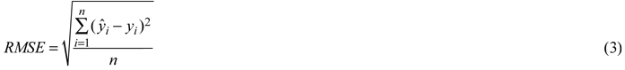
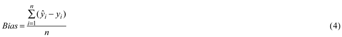
where![]() denotes the predicted variable and
denotes the predicted variable and![]() denotes the observed variable. The RMSE and bias calculations were performed for the forest variables basal area weighted mean tree height (BWH), basal area weighted mean tree diameter (BWD), mean stem volume per hectare (MSV), basal area (BA) and stand mean age (MA). Next, the RelRMSE and RelBias were calculated (Eq. 5 and 6):
denotes the observed variable. The RMSE and bias calculations were performed for the forest variables basal area weighted mean tree height (BWH), basal area weighted mean tree diameter (BWD), mean stem volume per hectare (MSV), basal area (BA) and stand mean age (MA). Next, the RelRMSE and RelBias were calculated (Eq. 5 and 6):


where![]() denotes the mean of the observed variable of each evaluation plot and the RMSE and bias were calculated according to Eq. 3 and 4.
denotes the mean of the observed variable of each evaluation plot and the RMSE and bias were calculated according to Eq. 3 and 4.
2.5 Accuracy of stem diameter distribution
The accuracy of the estimated stem diameter distributions was assessed using the total variation distance index (Levin et al. 2009) computed for each of the evaluation plots (40 m radius) using the diameter classes’ absolute differences (e, Eq. 7). Overall there were 20 diameter classes, where the width of each diameter class was 2 cm.

where ej is the error in diameter class j, P( xj ) is the observed relative frequency of diameter class j of the observed alternative, and Q( xj ) is the relative frequency of diameter class j in the diameter distribution predicted by the other alternatives, i.e., S500, S250, S91, subS91, syst10m and syst5m. The errors of the estimated diameter distributions were multiplied by ½ to scale the error index between 0 and 1, where 0 represented a perfect match of the two compared distributions. P( xj ) was calculated by dividing the observed number of trees in each class by the observed total number of trees in the evaluation plot. Q( xj ) was calculated by dividing the number of predicted trees in each class by the total number of predicted trees in the evaluation plot. The evaluation plot level error e was defined as the sum of the diameter class error ej. The total variation distance was used as a measure of the degree of the diameter distribution errors that were independent of the total number of trees.
2.6 Calculation of suboptimal losses
The evaluation plot data for each of the seven alternatives (one observed and six imputed) were imported as tree lists into the Heureka system (Wikström et al. 2011). The system was used to simulate and evaluate different possible treatment for 20 five year periods (i.e., 100 years). The optimal management strategies providing the highest Net Present Value (NPV) were selected for all alternatives. The two first planning period management actions selected in the imputation alternatives were then applied to the forest data for the observed alternative and the subsequent NPVs calculated. The differences between the NPV of the observed alternative to the NPV of the applied programs on the forest information in the observed alternative were considered to be the suboptimal losses (Saad et al. 2014). Only the two first periods (10 years) of the management actions were used from the imputed alternatives because it was assumed that in the future, new and improved information would likely be available (Holmström et al. 2003). Information on the suboptimal losses can help forest planners to determine whether it is cost effective to change the sampling design, e.g., using the LPM sampling design instead of the traditional systematic plot sampling design.
3 Results
The accuracy validations of the reference plot data imputation to the evaluation plots were presented in terms of the RelRMSE and RelBias values (Eq. 5 and 6) for the five key forest variables BWH, BWD, MSV, BA and MA in the six imputations alternatives (Table 3).
| Table 3. Summary of the relative root mean square error (RelRMSE) and relative bias (within parenthesis) values, for the forest variables basal area weighted mean tree height (BWH), basal area weighted mean tree diameter (BWD), mean stem volume per hectare (MSV), basal area (BA) and stand mean age (MA), indicating the accuracy of the airborne laser scanning based imputation of the reference plot data to the 40 m radius evaluation plots for the six different estimated alternatives. | |||||
| Alternative | RelRMSE (%) | ||||
| BWH | BWD | MSV | BA | MA | |
| S500 | 9.6(–6.8) | 8.7(5.7) | 24.7(9.9) | 26.8(17.1) | 21.6(–7.7) |
| S250 | 10.8(–7.8) | 9.0(4.7) | 18.6(–2.1) | 16.2(8.1) | 20.4(–9.6) |
| S91 | 13.6(–9.5) | 10.7(3.4) | 23.3(–3.1) | 20.5(8.5) | 28.7(–13.2) |
| subS91 | 10.6(–7.0) | 11.9(5.8) | 38.8(11.9) | 38.2(19) | 25.0(–7.9) |
| Syst10m | 8.4(–5.6) | 8.0(0.0) | 23.8(–10.6) | 18.3(–8.0) | 20.0(–4.0) |
| Syst5m | 10.1(–8.0) | 8.7(–4.2) | 27.3(–14.9) | 18.3(–8.0) | 23.1(–6.2) |
The results showed that the bias in most cases was moderate except for BA in the S500 and subS91 alternatives, which showed a high positive BA bias. In both the latter cases, there was also a negative BWH bias, resulting in a moderate MSV bias. High bias was also reflected in the RelRMSE values.
Among the LPM alternatives, either S500 or S250 gave the lowest RelRMSE for all variables. S500 gave the lowest values for BWH and BWD, whereas S250 gave the lowest values for the other variables. S91 and subS91 performed worse than the best performing (lowest RelRMSE) alternatives S500 or S250 for all variables. Also when comparing with the worst (highest RelRMSE) among S500 and S250 the S91 and subS91 alternatives performed worse or close to (BWH and MSV) except for BA (S500 26.8% and S91 20.5%, respectively). When comparing S91 and subS91 (in the latter case, one reference plot in each micro stand), subS91 performed worse or much worse than S91 for three variables (BWD, MSV and BA). Among the systematic design alternatives, Syst10m gave a lower or equal RelRMSE then Syst5m for all variables.
When comparing the LPM alternatives with the systematic design alternatives, the latter gave a lower RelRMSE for three (BWH, BWD and MA) out of the five variables. When comparing the approaches with a similar number of plots and the same plot radius, i.e., S250 vs. Syst5m, the RelRMSE was roughly equal except for MSV, for which S250 showed a much lower value (18.6% vs. 27.3% for Syst5m).
Error indices (Eq. 7) of the estimated stem diameter distributions are presented in Table 4. For the LPM alternatives, the mean error indices increased with decreasing number of reference plots; S91 and subS91 showed equal mean error indices. Among the systematic sampling design, Syst10m gave a lower mean error index than Syst5m, and Syst10m also performed better than the micro stand and LPM alternatives. The alternatives with roughly the same number of plots and plot radius, i.e., S250 and Syst5m, gave similar mean error indices.
| Table 4. Summary of error indices of the estimated diameter distributions indicating the accuracy of the estimated diameter distributions using the two different sampling methods, local pivotal method and systematic, with different reference plot intensity. The index value 0 indicates a perfect match of the compared distributions. | ||||
| Alternative | Error indices of the estimated diameter distributions - total variation distance index | |||
| Mean | Minimum | Maximum | sd* | |
| S500 | 0.27 | 0.12 | 0.64 | 0.11 |
| S250 | 0.29 | 0.15 | 0.62 | 0.1 |
| S91 | 0.35 | 0.13 | 0.69 | 0.12 |
| subS91 | 0.35 | 0.2 | 0.54 | 0.1 |
| Syst10m | 0.24 | 0.12 | 0.48 | 0.08 |
| Syst5m | 0.28 | 0.15 | 0.53 | 0.09 |
| * sd: standard deviation | ||||
NPVs were calculated by the Heureka DSS using a 3% real interest rate. As described in the previous section, the suboptimal loss was calculated for each imputation alternative. The suboptimal losses using the LPM sampling design were 47, 62, 39 and 28 euros ha–1 for the S500, S250, S91 and subS91 alternatives, respectively. The suboptimal losses using the systematic sampling design were 61 and 63 euros ha–1 for the syst10m and syst5m alternatives, respectively. The alternative subS91 yielded the lowest suboptimal loss but the highest error index of the estimated diameter distributions (along with S91) and the highest mean stem volume RelRMSE.
4 Discussion
In this study, a novel data acquisition approach was used that combines the concept of micro stands and the LPM sampling design using ALS data as auxiliary data. The nonparametric MSN method was then used for the imputation based on two different sets of reference plots and a total of six different imputation alternatives. The allocation of reference plots among micro stands in the first set of reference plots and the location of the plots within the micro stands were carried out using the recently developed LPM sampling design. In both cases, ALS data were used as auxiliary information (imputation alternatives 2–5). The latter approach was compared with a traditional layout of reference plots in a square grid over the forest area, which made up the second set of reference plots (imputation alternatives 6–7). The data quality (Table 3 and 4) of the six estimated alternatives was compared and the suboptimal losses due to inoptimal treatment decisions were calculated using the Heureka DSS.
According to the results – RMSE, bias (Table 3), stem diameter distribution error indices (Table 4) and suboptimal losses – none of the sampling designs, i.e., LPM vs. systematic, showed a clear advantage over the other. Both the random and systematic errors showed large variations among the imputation alternatives. This was, to some degree, expected because the inference method does not utilize weighting (i.e., smoothing of several observations), unlike in the kMSN method (k > 1), to reduce the prediction errors. Thus, the few extreme reference observations may have had a very large influence. Among the systematic sample design alternatives, i.e., syst10m and syst5m, the RelRMSE, stem diameter distribution error index and suboptimal loss were smaller for the 10 m radius reference plots than for the 5 m radius plots, indicating higher accuracy for syst10m as expected. Among the alternatives using the LPM sampling design, i.e., S500, S250, S91 and subS91, the stem diameter distribution error index increased as the number of reference plots decreased, indicating decreasing accuracy. This pattern of lower estimation accuracy (as for the error index) as the sample size was reduced did not hold for all estimated variables regarding the values of the RelRMSE, RelBias (Table 4) and suboptimal loss. Some extreme values might have had a large effect on the RelRMSE of the estimated variables owing to the low number of evaluation plots (n = 30). If the number of evaluation plots had been larger, the effect of a few extreme values on the RelRMSE and RelBias for some imputation alternatives would have been smaller.
The six different imputation alternatives corresponded to different sample designs, number of reference plots and plot radii. For comparing the different sampling designs, i.e., LPM vs. systematic, the alternatives S250 and syst5m were the most suitable because these alternatives had roughly the same number of reference plots and plot radius, i.e., 5 m. The differences between the S250 and syst5m alternatives in the stem diameter distribution error indices and suboptimal losses were very small. The differences in the RelRMSE were larger, especially for MSV. For this variable, the RelRMSE was notably lower for the S250 alternative compared to the syst5m alternative, indicating that the LPM sampling design measured the volume more accurately than the systematic sampling design given approximately the same number and size of reference plots.
The differences in the suboptimal losses were not very large (259 euros ha–1 to 584 euros ha–1), but as the suboptimal losses did not follow the trends in accuracy of the forest variable estimations, these figures is quite uncertain. The suboptimal losses for each alternative were calculated by observing the individual suboptimal loss of each unit, i.e., the 30 evaluation plots. The proportion of units contributing to the suboptimal loss was 16–23% in the different alternatives. This means that 77–84% of the units in the different alternatives showed zero suboptimal losses as the same treatments were proposed for the imputed alternatives as for the observed alternative. Several units gave large suboptimal losses, which consequently had a large effect on the average suboptimal loss for each alternative as the number of units (evaluation plots) was low. Given a higher number of evaluation units (say 1000), the extreme values would have had a smaller effect on the average suboptimal loss. Thus, the fluctuations of the suboptimal losses among the alternatives probably reflect the low number of evaluation plots used.
The sample procedures considered in this study were performed once when reducing the sample size in the LPM design and when selecting the sample in the systematic sample design. Sampling errors (Holmström et al. 2003; Islam et al. 2010) associated with reducing the sample size (Maltamo et al. 2009), were not considered and there was no attempt to repeat the procedure as it was deemed too laborious and time consuming; the expected time for completing the calculation of the suboptimal losses for repetitions of the procedure was considered unreasonable.
The reference plots sampled following the LPM sampling design suffered from low accuracy of the plot location due to the Global Navigation Satellite System (GNSS) used, whereas the plot locations of the reference plots sampled following the systematic sampling design had a high GNSS accuracy. This could of course have had a large effect on the estimations of the RelRMSE, stem diameter distribution index error and suboptimal loss. Unfortunately, this effect could not be quantified as the positioning accuracy was not known in the study. Even though the positions of the LPM reference plots were not accurate, comparable results to the systematic sampling design were obtained, which indicates that the LPM design offers further potential that was not realized in this study.
In practice a systematic sample design is seldom used today and instead typically stratified approaches are used. As a stratified approach includes several (subjective) factors – most of all the number of strata and which variables to base the stratification on – it is less appropriate in a research setting like the present study. Further, as mentioned the systematic sample design reference plots’ were originally designed to be applicable in several different remote sensing research projects. Although both sampling designs, i.e., LPM and systematic, was performed in a research setting without any detailed measurement of time consumption, the LPM sampling design was found to be faster compared to the systematic sampling design. If a cost-plus-loss analysis were to be performed, the LPM sampling design would likely be favored over the systematic sampling design. That is because of time savings when moving between the plots, e.g., shorter routes and quick measures. Thus, it would be invaluable in future studies to reconsider the use of LPM design sampling with more accurate GNSS and compare it with existing methods. As the different alternatives did not show significant differences in the obtained values for the suboptimal loss, RelRMSE (Table 3, except for subS91 in MSV and BA) and error index of the estimated stem diameter distributions (Table 4), S91 may be considered in this case to be the favorite alternative; the cost of data acquisition in S91 was comparably very low and was capable of being completed within a shorter time compared to other alternatives.
For future studies would be of interest to perform a cost-plus-loss analysis in order to test whether the LPM sampling design is cost efficient sample design. The non parametric estimation technique, kMSN, could be suitable to utilize weighting if k would be larger than 1, this could lead to reduction in the prediction errors. It is recommended to plan proper sample for the future studies in order to keep control over all factors that can affect the remote sensing techniques.
Overall, the results of this study show the great potential for improving data acquisition methods by employing the new sampling design LPM and micro stand delineation techniques. One reason for choosing the LPM sampling design is its cost efficiency compared to the systematic sampling design.
Acknowledgment
This study was financed by “The Swedish Forest Society Foundation” (Skogssällskapet). The ALS data and field inventories were financed by Hildur and Sven Wingquist foundation. The authors also thank Dr. Anton Grafström for valuable advice concerning the used sampling methods.
References
Bettinger P., Boston K., Siry J.P., Grebner D.L. (2009). Forest management and planning. Academic Press, New York. p. 67.
Duvemo K., Lämås T. (2006). The influence of forest data quality on planning processes in forestry. Scandinavian Journal of Forest Research 21(4): 327–339. http://dx.doi.org/10.1080/02827580600761645.
Grafström A., Ringvall A.H. (2013). Improving forest field inventories by using remote sensing data in novel sampling designs. Canadian Journal of Forest Research 43(11): 1015–1022. http://dx.doi.org/10.1139/cjfr-2013-0123.
Grafström A., Lundström N.L.P., Schelin L. (2012). Spatially balanced sampling through the pivotal method. Biometrics 68(2): 514–520. http://dx.doi.org/10.1111/j.1541-0420.2011.01699.x.
Holmström H., Kallur H., Ståhl G. (2003). Cost-plus-loss analyses of forest inventory strategies based on kNN assigned reference sample plot data. Silva Fennica 37(3): 381–398. http://dx.doi.org/10.14214/sf.496.
Hyvönen P, Pekkarinen A, Tuominen S. (2005). Segment-level stand inventory for forest management. Scandinavian Journal of Forest Research 20(1): 75–84. http://dx.doi.org/10.1080/02827580510008220.
Islam M.N., Kurttila M., Mehtätalo L., Pukkala T. (2010). Inoptimality losses in forest management decisions caused by errors in an inventory based on airborne laser scanning and aerial photographs. Canadian Journal of Forest Research 40(12): 2427–2438. http://dx.doi.org/10.1139/X10-185.
Kangas A.S. (2010). Value of forest information. European Journal of Forest Research 129(5): 863–874. http://dx.doi.org/10.1007/s10342-009-0281-7.
Koch B, Straub C, Dees M, Wang Y, Weinacker H. (2009). Airborne laser data for stand delineation and information extraction. International Journal of Remote Sensing 30(4): 935–963. http://dx.doi.org/10.1080/01431160802395284.
Levin D.A., Peres Y., Wilmer E.L. (2009). Markov chains and mixing times. Providence, RI: American Mathematical Society. p. 48.
Maltamo M., Næsset E., Bollandsås O.M., Gobakken T., Packalén P. (2009). Non-parametric prediction of diameter distributions using airborne laser scanner data. Scandinavian Journal of Forest Research 24(6): 541–553. http://dx.doi.org/10.1080/02827580903362497.
Moeur M., Stage A.R. (1995). Most similar neighbor: an improved sampling inference procedure for natural resource planning. Forest science 41: 337–359.
Olla H. (1990). Computer aided forest stand delineation and inventory based on satellite remote sensing. The usability of remote sensing for forest inventory and planning. Proceedings from SNS/IUFRO workshop in Umeå 26–28 February 1990.
Olofsson K., Holmgren J. (2014). Forest stand delineation from lidar point-clouds using local maxima of the crown height model and region merging of the corresponding Voronoi cells. Remote Sensing Letters 5(3): 268–276. http://dx.doi.org/10.1080/2150704X.2014.900203.
Söderberg U. (1992). Functions for forest management. Height, form height and bark thickness of individual trees. Report 52. Department of Forest Survey, Swedish University of Agricultural Sciences, Umeå, Sweden. 87 p. [In Swedish with English summary].
Packalén P., Maltamo M. (2007). The k-MSN method for the prediction of species-specific stand attributes using airborne laser scanning and aerial photographs. Remote Sensing of Environment 109(3): 328–341. http://dx.doi.org/10.1016/j.rse.2007.01.005.
Pippuri I., Kallio E., Maltamo M., Peltola H., Packalen P. (2012). Exploring horizontal area-based metrics to discriminate the spatial pattern of trees and need for first thinning using airborne laser scanning. Forestry 85(2): 305-314. http://dx.doi.org/10.1093/forestry/cps005.
Saad R., Wallerman J., Lämås T. (2014). Estimating stem diameter distributions from airborne laser scanning data and their effects on long term forest management planning. Scandinavian Journal of Forest Research 30(2): 186-196. http://dx.doi.org/10.1080/02827581.2014.978888.
Wikström P., Edenius L., Elfving B., Eriksson L.O., Lämås T., Sonesson J., Öhman K., Wallerman J., Waller C., Klintebäck F. (2011). The Heureka forestry decision support system: an overview. Mathematical and Computational Forestry & Natural-Resource Sciences 3: 87–94.
Total of 19 references.
Send to email
