Annika Kangas  ,
Mari Myllymäki,
Lauri Mehtätalo
,
Mari Myllymäki,
Lauri Mehtätalo
Understanding uncertainty in forest resources maps
Kangas A., Myllymäki M., Mehtätalo L. (2023). Understanding uncertainty in forest resources maps. Silva Fennica vol. 57 no. 2 article id 22026. https://doi.org/10.14214/sf.22026
Highlights
- Forest resources maps without uncertainty assessment may lead to false impression of precision
- Suitable tools for visualization of map products are lacking
- Kriging method provided accurate uncertainty assessment for pixel-level predictions
- Quantile random forest algorithm slightly underestimated the pixel-level uncertainties
- With simulation it is possible to assess the uncertainty also for landscape-level characteristics.
Abstract
Maps of forest resources and other ecosystem services are needed for decision making at different levels. However, such maps are typically presented without addressing the uncertainties. Thus, the users of the maps have vague or no understanding of the uncertainties and can easily make wrong conclusions. Attempts to visualize the uncertainties are also rare, even though the visualization would be highly likely to improve understanding. One complication is that it has been difficult to address the predictions and their uncertainties simultaneously. In this article, the methods for addressing the map uncertainty and visualize them are first reviewed. Then, the methods are tested using laser scanning data with simulated response variable values to illustrate their possibilities. Analytical kriging approach captured the uncertainty of predictions at pixel level in our test case, where the estimated models had similar log-linear shape than the true model. Ensemble modelling with random forest led to slight underestimation of the uncertainties. Simulation is needed when uncertainty estimates are required for landscape level features more complicated than small areas.
Keywords
autocorrelation;
ensemble modelling;
kriging;
quantile;
random forest;
sequential Gaussian simulation
-
Kangas,
Natural Resources Institute Finland (Luke), Bioeconomy and environment, Yliopistokatu 6, 80101 Joensuu, Finland
 https://orcid.org/0000-0002-8637-5668
E-mail
annika.kangas@luke.fi
https://orcid.org/0000-0002-8637-5668
E-mail
annika.kangas@luke.fi
-
Myllymäki,
Natural Resources Institute Finland (Luke), Bioeconomy and environment, Latokartanonkaari 9, FI-00790 Helsinki, Finland
https://orcid.org/0000-0002-2713-7088
E-mail
mari.myllymaki@luke.fi
-
Mehtätalo,
Natural Resources Institute Finland (Luke), Bioeconomy and environment, Yliopistokatu 6, 80101 Joensuu, Finland
https://orcid.org/0000-0002-8128-0598
E-mail
lauri.mehtatalo@luke.fi
Received 9 December 2022 Accepted 24 May 2023 Published 31 May 2023
Views 87816
Available at https://doi.org/10.14214/sf.22026 | Download PDF

1 Introduction
Maps are often utilized as tools in science-policy interfaces such as Reducing Emissions from Deforestation and Forest Degradation in Developing Countries (REDD+), Intergovernmental Panel on Climate Change (IPCC) or Intergovernmental Science-Policy Platform on Biodiversity and Ecosystem Services (IPBES) to communicate state of environments to policy makers (Ojanen et al. 2021). Pan-European maps would be beneficial in monitoring the development towards targets in various EU-level policies (Lier et al. 2021). For instance, mapping the aboveground biomass of tropical forests is essential both for implementing conservation policies and reducing uncertainties in the global carbon cycle (Mitchard et al. 2013). The state of the environment in such a map is typically a model prediction, based on remotely sensed information for each pixel or cell in the area. In science-policy interface it is important that the maps used are accurate, and having for instance, several maps of varying quality from the same area and theme may be confusing, and a source of distrust among stakeholders (Ojanen et al. 2021).
In general, maps are needed for local decision making (Kangas et al. 2018), as well as local monitoring of the state of environment, for instance for sustainability considerations (Katila et al. 2020). In Finland, the first national-level thematic maps describing the status of forests were published already in the 1990’s (Tomppo 1996), and currently such maps are produced in many other countries as well (Baccini et al. 2011; Saatchi et al. 2011; Freeman and Moisen 2015; Nord-Larsen et al. 2017; Nilsson et al. 2017; Hauglin et al. 2021). However, use of maps is not restricted to forest resources, but all ecosystem services benefit from map data (Burkhart et al. 2012; Maes et al. 2012).
While maps are useful in many different decision-making contexts, inaccuracies in a map may lead to wrong conclusions and through that to suboptimal decisions. There exist examples where a published map or an analysis based on such a map has led to heavy criticism due to the inherent (reported or unreported) uncertainties. For instance, Ceccherini et al. (2020), published an analysis where they argued a dramatic rise in forest harvest levels in Europe, especially in Sweden and Finland: 69% in biomass and 43% in area between two periods, 2010–2015 and 2016–2018. This analysis was based on a map depicting tree cover loss (Global Forest Watch, see Hansen et al. 2013). It was subjected to severe critic (Palahi et al. 2021 and Wernick et al. 2021 among others). Breidenbach et al. (2022) demonstrated that the maps based on remote sensing contradict with extensive field-based national forest inventory data sets. According to critics, the used map of tree cover loss is not suitable for the task in the first place, as it acknowledges only abrupt losses in the canopy cover, not the gradual forest growth. The published critics also pointed out that in the earlier period a smaller part of changes were depicted. Breidenbach et al. (2022) concluded that it is not the harvests, but the ability to detect harvests that has increased abruptly. At the end of public discussion, Ceccherini et al. (2022) concluded that remote sensing-based maps on land use change are useful mainly as tools to plan field inventories.
The REDD+ program requires accurate information of the forest degradation and loss. In many countries, remote sensing -based maps are the only option to achieve such information. In 2008, Bacchini et al. published a map for sub-Saharan Africa, where they claimed a very good accuracy, with a map explaining 82% of the variability of the above-ground biomass (AGB). Only a couple years later, Mitchard et al. (2011) compared the map data to their own field plots and argued that only a very weak correlation with the map was observed, with 28% of the variation explained in the independent test data. They concluded that Bacchini et al. (2008) had too poor-quality data with a too limited spatial extent for modelling, which explains the observed poor quality. For instance, part of the plots used in modelling were derived from a land cover map rather than actual measurements. Mitchard et al. (2011) conclude that a good quality map requires good quality field data drawn from across the spatial extent and ecological variability of the prediction area, and accuracy assessments done against truly independent datasets. Meyer and Pebesma (2021, 2022) also stress the spatial distribution of training data as a pre-requisite for applicable maps.
In Finland, Mikkonen et al. (2018, 2020) published maps describing deadwood potential of Finnish forests. This analysis was heavily criticized by other researchers (Kangas and Mehtätalo 2021), as it was based on simulated deadwood data and an extrapolation of a 5th degree polynomial model. However, the maps based on this model had already been used in addressing the quality of the Finnish nature conservation programme Metso without any consideration of uncertainties. This analysis was carried out even though the original authors of the map suggested that the product should only be used as prior information to find mature stands for field assessment of the conservation value.
In other occurrences, researchers have compared maps produced in different campaigns, and found that the maps are not agreeing as well as the users might hope or believe. For instance, Zhang et al. (2019) compared maps produced for ABG in many different studies and for all the continents. They concluded that the forest biomass datasets were almost entirely inconsistent. Schulp et al. (2014) compared four maps of ecosystem services at the European level. The produced maps strongly disagreed, for instance, on the potential of climate regulation in Sweden and Finland, despite of the large proportion of forests in both countries (70% and 74%, respectively). Eigenbrod et al. (2010) generalized sample-based data of three ecosystem services in two different ways. When looking at hotspots (the best 10% of the area regarding the indicator in question), the two maps were overlapping in 23% of cases for biodiversity, 17% for recreation and 62% for carbon storage. Mitchard et al. (2013) compared two maps for AGB in Africa, which were based on the same input data (GLAS laser scanning from a satellite), but a different methodology. They concluded that there were substantial differences between the maps, and even the direction of change was inconsistent. When aggregated to country level, the maps converged better, meaning that location uncertainty is important. Eigenbrod et al. (2010) also concluded that while comparisons between the maps are interesting, they are of limited use in either confirming the validity of the mapping approach or stating whether one map should be used preferentially to the other. Thus, analytical methods to address the map uncertainty are needed.
The aim of this paper is to highlight the importance of map uncertainty and to review methods to deal with map uncertainty and to visualize it. Two of the reviewed methods, namely quantile random forest and kriging, are tested and illustrated in a dataset with 17 laser scanning features and a simulated response variable. This work is carried out to improve the understanding of the uncertainties among the users and producers of the maps.
2 Map uncertainty
2.1 Types of map uncertainty
Map uncertainty means that we can address the local error, i.e. to predict the uncertainty at each location separately (Vaysse and Lagacherie 2017; Kasraei et al. 2021). It can be interpreted as estimating prediction error variance for a new observation in regression analysis. Since all model predictions, irrespective of the modelling method, are inevitably model-based and conditioned on the modelling data set, it can also be interpreted as model-based inference at pixel level. Yet, the term “model-based inference” is often restricted to an approach of making population-level or domain-level inferences based on an observed sample (see Särndal et al. 1992) rather than estimating observation-level uncertainties that are important in a mapping exercise.
Nevertheless, another important case of map uncertainty is to predict the uncertainty simultaneously at several points or at a given sub-area (spatial uncertainty, Goovaerts 2001). This could be, for instance, a field, a lake or a forest stand. Since the measurement units are typically smaller than such sub-areas, aggregation of the predictions is required (Goovaerts 2001). In this case, the spatial uncertainty can be estimated using model-based inference in a small-area estimation context (Magnussen and Breidenbach 2017; Astrup et al. 2019), for instance using block-kriging (Schabenberger and Gotway 2005).
The uncertainty can also be looked from another perspective, location error, meaning there is uncertainty as to where a certain resource is located. For instance, we would like to know where the old-growth forests, the forests with highest biodiversity or the forests with greatest volume of deadwood are located. We might, for instance, wish to delineate an area with a, say, 95% probability to have at least a specified target level, say 20 m3, of deadwood. From this point of view, it is possible for instance to assess the probability of finding a given resource at some location using a classification algorithm or classifying the model predictions. In an area context, the joint probability of the units fulfilling the condition would be needed. While the classification accuracy is also a highly important topic, it is not covered in this article, but the readers are referred to Olofsson et al. (2014).
The location of a given resource can be interpreted as a landscape level feature. Other landscape level features of interest may include, for instance, the sizes of patches of a given habitat, the distances between those habitats or connectivity of the habitats in the landscape. In addition to the pixel-level or small-area level uncertainties, we should be able to also assess the uncertainties of such landscape features, but to the knowledge of the authors no literature regarding such assessments related to forests has been published.
2.2 Sources of map error
As the thematic maps are essentially predictions with locations, the map uncertainty stems from the model behavior. In statistical literature, the best predictor of a random variable Y using observations of random variable X is the conditional expectation E(Y | X) (Christensen 2011). In this context, X includes the independent variables (predictors) of the applied regression model, which are thought as random (Mehtätalo and Lappi 2020: p. 309). Depending on the context, the predictors can also be assumed as fixed.
We assume that the true values at the pixel locations of a map are generated by a regression model, so that the observed values can be written as:
![]()
where e is a residual error. The marginal variance of y is therefore (Mehtätalo and Lappi 2020: p. 25, Eq. 2.46):
![]()
whereas that of the best prediction includes only the term var(E (Y | X)). Thus, the uncertainty of the best prediction is closer to the Berkson case where the true value y varies randomly around its estimate ![]() and errors are uncorrelated with
and errors are uncorrelated with ![]()
![]()
than to the classical measurement error model with:
![]()
where measurement errors are uncorrelated with true values (Mehtätalo and Lappi 2020: p. 384). In a case of Berkson type error (3), the variation across the map of ![]() is always less than the true variation in y (var(
is always less than the true variation in y (var(![]() ) < var(y)), while in traditional measurement error model (4) inequality is to other direction (var(
) < var(y)), while in traditional measurement error model (4) inequality is to other direction (var(![]() ) > var(y)). Berkson type errors are common for instance for controlled regressors (Seber and Wild 1989) or visual assessments (Kangas et al. 2004). It is important to note the error type, especially when looking for the extreme values of any forest characteristics based on different prediction or measurement procedures. Estimation errors of the model parameters will also contribute to the above-specified formulas but do not change the conclusions.
) > var(y)). Berkson type errors are common for instance for controlled regressors (Seber and Wild 1989) or visual assessments (Kangas et al. 2004). It is important to note the error type, especially when looking for the extreme values of any forest characteristics based on different prediction or measurement procedures. Estimation errors of the model parameters will also contribute to the above-specified formulas but do not change the conclusions.
The most evident source of map uncertainty is the variance of the residual errors of the model used, var(ei), which describes the uncertainty due to the relationship between the response and the selected predictors within the modelling data, estimated using the residuals of the model. The variance is typically assumed constant, var(ei) = σ2 but may also be modelled as a function of the prediction or one or more predictors to account for a heteroscedasticity of the error. If the residual errors are assumed independent and identically distributed, as is usually assumed, mapping the residual uncertainty does not provide any useful information for users. Even when the residual errors are spatially correlated, the expected uncertainty at each location is the residual error variance of the model.
Generally, the uncertainty due to the residual errors is random error. However, when there is spatial correlation (either in the form of random area-effects or distance-dependent correlation), it needs to be considered when estimating the uncertainty of aggregates or means over an area. The correlated errors will introduce domain-level bias (e.g. within a forest stand), which need to be accounted for in the analysis (Magnussen and Breidenbach 2017).
Another source of uncertainty is the parameter estimation error. In principle, the parameter estimation errors produce random uncertainty, as the least squares or maximum likelihood estimators are unbiased. Across all potential data sets, the parameter estimations errors are random. Yet, for a given modelling data set these errors are fixed and behave like bias in the predictions (Mehtätalo and Lappi 2020). This source of uncertainty can be assessed analytically, with Monte Carlo simulation using the distributions of the estimated parameters or with repeating the modelling task with repeated samples of the available data (bootstrapping, Efron and Tibshirani 1996). Alternatively, a Bayesian statistics approach can be used and then the parameter uncertainties are represented in the posterior distributions of the parameters, which are constructed from the prior distributions (the knowledge prior to the experiment) and the maximum likelihood (i.e. data).
Third source of uncertainty is due to model selection. This source includes the uncertainty related to deciding the number of predictors included and selecting the best predictors from among several potential predictors. It also includes the uncertainty due to selecting the model form used from among different model families, for instance the selection between linearized and non-linear model form. This effect can be assessed by calculating the variation from an ensemble of potential models. Of course, uncertainty due to potential predictors that are known to be important, but for which with no data are not observed, always remains unattainable. Likewise, uncertainty of extrapolating the model outside data available may cause systematic error, which is unattainable unless independent data can be achieved. Unless the model form correctly describes the population for which the model is applied, model selection error may be an important source of bias in the map predictions.
In addition to the prediction errors, there may also be errors in the input variables, for instance due to measurement or sampling errors (Peters et al. 2009). If the measurement errors are similar in the modelling data and data used in applications, they increase the prediction variance but do not introduce systematic error (Kangas 1998). If the remote sensing features are used as predictors, co-location errors, light conditions, camera and scanner quality that are not similar in the modelling and application phases can cause systematic errors that are not easily considered in the accuracy assessment (Saarela et al. 2016).
It is important to note that all the mentioned sources of uncertainty can, depending on the case, cause both systematic and random uncertainty. It is also important to note that all systematic errors in the predictions originally stem from one of these sources.
3 Methods to deal with map uncertainty
3.1 Analytical analysis of modelling errors
The number of papers describing the map uncertainties in different fields has rapidly increased in the recent decade. Yet, methods to address the uncertainty have been available already for decades (Goovaerts 2001).
The most obvious approach is to utilize the error estimates available from fitting a model to observed data analytically. In a case of parametric modelling, the deterministic part of the characteristics may be modelled using linear or non-linear regression whereas the stochastic part of variation is modelled with assumptions concerning the distribution of residuals. The prediction variance for a new observation y0 is a combination of the estimation error of model parameters and the variance of the residual errors (Mehtätalo and Lappi 2021: p. 126). For the linear model y = Xβ + e where var(e) = V is the variance-covariance matrix of the residual errors describing possible heteroscedasticity and autocorrelation structure,
![]()
where var(e0) is the residual error variance for a new observation y0 with predictor values x0 and X is the matrix containing all observed predictor values (which are now treated as fixed). This approach assumes the selected model as such is correct, and thus model selection errors are not included. In case of a non-linear model, the calculations require linearizing the model with, e.g., a Taylor series approach (Saarela et al. 2020). Model input variable errors can also be included analytically.
The existing observations can be used to improve the linear model prediction corresponding the location of interest. Such approach, which can be understood as kriging prediction of residuals, is useful if at least some existing observations are so close to the location of interest that the correlations are practically non-zero. The variance of prediction errors then is (Mehtätalo and Lappi 2021: p. 129):

where c = cov(e, e0) is the covariance matrix between errors at existing observations and the new point. In kriging, this covariance is typically presented as a function of distance. The prediction variance is the sum of the estimation variance of the deterministic component and the prediction variance of the kriged residuals (Hengl et al. 2007; Szatmári and Pásztor 2019).
If the uncertainty is needed for an area rather than for a single point, it can be calculated analytically based on the covariances between the residuals of predictions at different points as (Kotivuori et al. 2020; Breidenbach et al. 2016):

where the variance of the mean prediction ![]() in the area i is estimated from the estimated variances of the parameters and the estimated covariances (or variances in case j = k) of the errors of each N pixels or cells within the area.
in the area i is estimated from the estimated variances of the parameters and the estimated covariances (or variances in case j = k) of the errors of each N pixels or cells within the area.
3.2 Simulation
Analysis of the uncertainties can be based also on simulation (Goovaerts 2001). In simulation, several equally probable realizations of the same model are produced. Simulations may be preferred in estimation of uncertainty, if in addition of the prediction variance, the distributions or variance of other interesting quantities are desired and not analytically known. Journel (1996) used the term stochastic imaging for the simulation approach, where repeated replications of the map are simulated from a geostatistical model and the pixel-level variation between the simulated maps is used for assessing uncertainty (Chiles and Delfiner 1999). Different sources of uncertainties can be included into the simulations. Thus, the approach can account both for the parameter and residual error uncertainties.
In the context of large area maps, efficient simulation algorithms are essential. If the repeated replications are produced using a sequential Gaussian simulation (sGs), the spatial autocorrelations can be accounted for through the spatial relationships of the units already visited (Goovaerts 2001; Plant 2019). The between-realization variation within each pixel approximates the analytical estimate of uncertainty, available for the Gaussian case.
3.3 Ensemble modelling
In addition to analytical prediction error formulas and simulation, a third approach to address pixel-wise uncertainties would be to utilize ensemble modelling (Nisbet et al. 2009). It means that rather than estimating one single model, a set of models is estimated, and the variation is calculated from this ensemble of potential models. This approach can be used to address the model selection error, but the ensemble is obviously limited to the data available. To gain benefits from an ensemble of models, the separate models need to be sufficiently diverse but still each of them should fulfill some minimum accuracy requirements. Indeed, convergence of similar models may convey a false sense of certainty (Bugman and Seidl 2020).
Random forest (RF) is a forest (or a set) of several regression trees. These trees are formulated so that they are as independent of each other as possible (Breiman 2001). It means that each tree in the forest uses a (bootstrap) sample of the data rather than all the data, as well as a sample of the available predictor variables to form diverse enough trees. As default, RF uses one third of available predictors in each sample. Together the trees use all the available information. Thus, the RF automatically handles with the parameter estimation uncertainty through sampling the data and model selection uncertainty through sampling the potential predictors. In the case of RF, the parameter uncertainty refers to the points of splits in the regression trees. Esteban et al. (2019) calls this kind of bootstrapping as internal. RF is directly applicable to both classification and regression problems.
In RF, the mean prediction of the various trees in the forest is used as the predicted value. According to Breiman (2001) the accuracy of the individual trees and the diversity of the different classification trees form an upper bound to the generalization error (prediction error). It is an upper bound, as none of the trees alone use all the available information. In the case of classification, the RF directly produces a probability of the target unit belonging to different classes, and this also measures the uncertainty of the classification. For instance, Peters et al. (2009) assessed the uncertainty in spatial interpolation of environmental variables using sGs and then utilized an RF ensemble model to classify the pixels into different vegetation types and the RF model metrics such as out-of-the-bag error to assess the classification uncertainty.
Esteban et al. (2019) used, in addition to the internal bootstrapping within RF also an external bootstrapping to produce an estimate of uncertainty. This means that they did not only produce different trees to the random forest using a bootstrap sample but used bootstrapping to repeat the whole random forest several times. It is notable that in their study the uncertainties from the external bootstrapping were markedly smaller than those from the internal bootstrapping. This is due to each tree in RF only including part of the data and predictors, while the mean prediction from each of the random forests in external bootstrapping uses the whole data.
Ensemble modelling and external bootstrapping approaches can also be used in connection to linear regression or a non-parametric method such as the k nearest neighbors (k-NN). If the predictors are resampled in a same way as in the RF ensemble model, the resulting uncertainty can be interpreted as upper bound following Breiman (2001).
In the Bayesian context, all predictors are typically included into the model, and continuous prior information can be provided on their effect, for example suggesting each variable to be probably unimportant, but with the possibility of larger effect if having predictive power (Gelman et al. 2013). In the Bayesian analysis, the model selection uncertainty can be included through so-called model averaging (Piiroinen and Vehtari 2017). Such averaging may, however, lead to rather computational approaches and their suitability for forest resource maps are still to be studied.
3.4 Quantile modelling
A fourth possible approach to quantify the map uncertainty is quantile regression, where a selected prediction interval can be estimated. In its original form, the quantile regression is based on linear regression, where each of the quantiles in the data is modelled using a linear model. The quantile regression can be interpreted to describe the residual error variation but ignore other sources of uncertainty. It is also possible to model the expected value using, for instance, k-NN and then use quantile regression to model the residual errors rather than the original variable. This allows for some flexibility into the model of the expected values (Kasraei et al. 2021): when the quantile regression is used to model the residual errors, the method can also be used in a case where the expected values are modelled with machine learning models such as RF or k-NN.
Quantile Random Forest (QRF) (Meinshausen 2006) is an extension of RF used to calculate the full conditional distribution of a prediction rather than only the conditional mean (Vaysse and Lagacherie 2017; Fouedjio and Klump 2019). Freeman and Moisen (2015), for instance, used QRF to assess the 5th, 50th and 95th quantiles of forest volume. The QRF also accounts for uncertainties in parameter estimation and predictor selection based on a model ensemble.
3.5 Proxies for uncertainty
It is also possible to address the quality of the predictions by analyzing the quality of data for the modelling task at hand. For instance, Meyer and Pebesma (2022) analyzed the effect of the distance between the target point and the observations in the k-NN method as a proxy measure of data quality: in areas where the distances are exceptionally long, the quality of predictions is likely to be poor. Sakar et al. (2022) used the degree of extrapolation needed for the application as a measure of quality of predictions. Extrapolation was defined to mean auxiliary variable values outside the convex hull defined by the auxiliary variable values from field plots, and the quality of predictions was classified as poor when the distance to this hull was more than mean distance between target point and observations plus two times the standard deviation of the distance. While such measures of data do not directly describe the variance of prediction errors like conventional uncertainty measures, they can advise the users of the usefulness of the maps.
3.6 Visualization of map uncertainty
For a traditional model with a single response and single predictor, the visualization of uncertainty is straightforward with the prediction intervals as a function of the predictor. For a map (i.e., two-dimensional representation) with x- and y-axis reserved for the coordinates, visualization of the uncertainty takes more imagination. Typically, the variation in the variable of interest is shown with a color, and other approaches are needed for the uncertainty. An obvious solution for this is to produce two maps, with one depicting the expected values, and another depicting the estimated uncertainty. This provides the visualization needed, but not simultaneously (Kaye et al. 2012). In digital settings, displaying two maps on top of each other may be more comprehensive than in traditional paper maps.
A commonly used method is to utilize bivariate maps, with the expected value presented as one dimension, and the uncertainty as another dimension (Kaye et al. 2012). The two dimensions can be described with the hue and intensity of the colors, for instance. Another possibility is to use the colors to describe the expected values, and the pattern or hatching to describe the uncertainty. One very popular approach is a bivariate choropleth model (Retchess and Brewer 2016; Mu and Tang 2019), which shows a classified response value and uncertainty for a given area, such as state or municipality. Another example of the visualization of map uncertainty simultaneously with the expected values is presented by Grêt-Regamey et al. (2013). They utilized a Bayesian network for a spatially explicit uncertainty assessment of carbon sequestration. They presented the expected values of the resulting classes with one color and represented the uncertainty of the result as a shading of that color, meaning the most uncertain values were represented with darker colors. This approach could be very useful, provided the number of classes is small. It might be challenging with fine resolution and fragmented variables.
4 Empirical test
4.1 Material
We made a small simulation experiment to illustrate the pixel-wise map uncertainties stemming from a fixed sample and from the variation between potential samples using two different modelling approaches, a log-linear model and QRF. The simulation experiment is needed to illustrate such uncertainties that cannot be depicted from a single sample, for instance the effect of sampling the data (between-sample variation). For the experiment, we utilized wall-to-wall data on a region of size about 5900 ha. It is a small part of a laser scanning campaign, serving as a means to visualize the results of the tests. This test data was available on a grid of 231 824 pixels, for which coordinates, 17 laser scanning features as well as 4 aerial photo features are available.
To have the “ground truth” or a “superpopulation model” (see Gregoire 1998) in the whole region, we simulated for each pixel i a volume with yi = exp(μi + ei) where μi is the predicted logarithm of volume from an external model and ei is the simulated random error with three different options, as specified in the following. This approach was selected to be able to simulate populations with a meaningful spatial pattern and autocorrelation structure (see Magnussen and Lehrman 2019 for an alternative approach). A spatial Copula (see Gräler and Pebesma 2011) was not an option due to lack of suitable field data: the measured field plots in the modelling data (see below) are so far from each other, that no autocorrelation was detected.
The external model was based on an independent modelling dataset of 1044 observations with field-measured values of total plot volume, basal area, mean diameter, and mean height, as well as a set of 190 laser scanning features (see Tuominen et al. 2018 and Balazs et al. 2022 for details). We modelled the plot-specific ln(y) using the best seven predictor model estimated with leaps package in R (Thomas Lumley based on Fortran code by Alan Miller, 2020), using the 17 features that were available both in the test and the modelling data. The following laser scanning features were used: The maximum height of the points, Height at which given percentiles (20% last echo, 45%, 65%, 70%, 90%, 95%) of vegetation points are accumulated (m), Proportion of vegetation points relative to all points (%, first and last echo), Skewness of the distribution of vegetation point heights, Proportion of points above mean height, Proportion of points having cumulated at 20% of the height from all points (%, last echo), Rumple index, Inner volume, SumEntropy (Haralick) of canopy surface model and Average intensity. Unless otherwise stated, the features were calculated from the first echoes. The selected model had residual standard error = 0.232 and multiple R2 = 0.897 in the modelling data. The coefficient estimates are presented in Table 1.
| Table 1. The parameter values for the model log(y) = β0 + βx1 + βx2 + βx3 + βx4 + βx5 + βx6 + βx7 + ε used for simulating the “true” values of volume for the simulation experiment. | |||
| Estimate | Std. Error | T Value | |
| Intercept | 1.537 | 0.142 | 10.86 |
| Hmax_f | 0.024 | 0.007 | 3.17 |
| Hq55_f | 0.028 | 0.010 | 2.80 |
| H90_f | 0.035 | 0.013 | 2.73 |
| Pveg_f | 0.010 | 0.001 | 18.33 |
| Hq20_l | 0.025 | 0.004 | 6.70 |
| Imean | –0.050 | 0.008 | –6.53 |
| Csm_sumEnt | 0.367 | 0.021 | 17.69 |
| The names of the variables are: The maximum height of the points, Height at which 55% and 90% of vegetation points are accumulated (m), Proportion of vegetation points relative to all points (%, first echo), Proportion of points having cumulated at 20% of the height from all points (%, last echo), Average intensity, SumEntropy (Haralick) of canopy surface model. | |||
The three different error distributions used to simulate e were: a) independent Gaussian errors with residual standard error from the model above, b) autocorrelated errors from a zero-mean Gaussian random field with exponential semivariogram model

with the nugget effect τ2 = 0.0318 and ϕ = 337 resulting in a practical range of 1011 meters and c) autocorrelated errors from a zero-mean Gaussian random field with the exponential semivariogram function (8) with τ2 and ϕ = 23 resulting in a practical range of 69 m. In all cases, the same variance σ2 = 0.0538 was assumed. In cases b and c, the simulation was carried out sequentially using a gstat R-package (Pebesma 2004).
As the modelling data did not allow calculating the autocorrelation for the volume, the range and relative nugget in option b) are based on the autocorrelation between errors of a model predicting one of the 17 laser scanning features (Average intensity) with other laser scanning features in a sample taken from the test data, and those in c) are based on Breidenbach et al. (2016). In case b), Average intensity thus served as a proxy for calculating the range and nugget relative to the variance, while the variance came from the model above. Option b) results in a correlogram

with 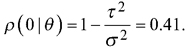 Consequently, we had three different populations with “ground truth” volume maps. The distribution of pixel-wise volumes for the case of independent errors a) is presented in Fig. 1. A part of maps from all three populations depicting the simulated logarithm of volume are presented in Fig. 2, to illustrate the effect of autocorrelation.
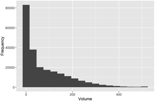
Fig. 1. The distribution of simulated “true” volumes (m3 ha–1) in the test area grid. The values > 500 m3 are all in the last class.
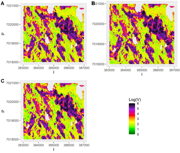
Fig. 2. The simulated “true” values of logarithm of volume in small part of the test data grid assuming a) independent errors b) autocorrelated errors with a long range (337 m) and large nugget effect and c) autocorrelated errors with no nugget effect and a short range (23 m). The scale is truncated at value 6.
4.2 Methods
We generated 100 random samples s of size m = 1000 from the simulated test data. To each of these samples s, we fitted a) a log-linear model for the volume with autocorrelated errors and the three best predictors out of the 17 possible predictors selected with the R package leaps (Thomas Lumley based on Fortran code by Alan Miller, 2020), and b) a quantile random forest (QRF) for the volume utilizing the R package quantregForest (Meinshausen 2017). The spherical semivariogram model was assumed for the log-linear model (even though the “true” semivariogram was exponential). These 100 samples were deemed as sufficient in this experiment these results remained stable over several repetitions of the calculations (see results for details).
Then, with each of the 100 fitted log-linear and QRF models, we predicted the volume at each pixel of the test data. For the linear model, kriging was carried out with the linear predictors and the fitted semivariogram model utilizing the R package gstat (Pebesma 2004; Gräler et al. 2016). The predicted volume was then obtained by ![]() where
where ![]() and
and ![]() are the prediction and prediction variance for the log volume. The variance was estimated using the variance of a log-normally distributed variable as
are the prediction and prediction variance for the log volume. The variance was estimated using the variance of a log-normally distributed variable as ![]() In QRF, the 50% quantile (median) was used as a prediction for each of the locations. The within-sample variation is represented with lower (2.5%) and upper (97.5%) quantiles.
In QRF, the 50% quantile (median) was used as a prediction for each of the locations. The within-sample variation is represented with lower (2.5%) and upper (97.5%) quantiles.
The variation between the 100 samples describes the model parameter estimation errors from different samples. To some extent it also describes model selection errors, i.e., the selection of the best predictors (predictors providing the minimum variance model in a given sample). The selected log-linear model was always the best three-predictor linear model with predictors selected from among all potential 17 predictors. Thus, the number of predictors is smaller than that in the superpopulation model used for generating the true data in order to depict potential model-selection error. Yet, the models from different samples are not independent of each other, and do not therefore represent a true ensemble of models. In QRF, there is variation in the models selected between the samples (external bootstrapping, Esteban et al. 2019). In addition, an ensemble of regression trees with a different set of potential predictors for each tree is used, and the estimated quantiles, i.e. the conditional distribution of the response variable reflects this within each simulation a between-model variation (internal bootstrapping, Esteban et al. 2019).
For both models, a relative standard error map was calculated from the variation among the 100 maps, relative to the expected value at each point. This represents the between-sample variation (not estimable from a single sample) that does not include the residual errors, but the variance due to model selection and parameter estimation for each sample.
A prediction interval was calculated for each pixel of the grid conditioned on each single sample. In QRF the prediction interval was simply the interval between the predicted 2.5% and 97.5% quantiles. For the linear model, the pixel-wise prediction interval was calculated from the estimated variance of the log-normal distribution, ![]() for each pixel as:
for each pixel as:
![]()
We also calculated the quantiles of the log-normal distribution but resorted to this simpler alternative in the example, as the resulting prediction intervals were nearly identical in these two cases.
These prediction intervals represent an uncertainty assessment estimable from a single sample. Then, the number of pixel-wise “true” volumes within the estimated prediction intervals were calculated. The quality of the spatial uncertainty assessment was addressed based on the mean number of observations within the prediction intervals, i.e. it describes how the pixel-wise prediction interval calculated from a single sample performed on average across the study region.
Visualizing the prediction interval in full requires two maps, one for the lower and another for upper bound. Therefore, in the following the uncertainty was instead visualized using a deviation from the expected value, ![]() for the linear model, and a half of the prediction interval (97.5% quantile – 2.5% quantile) for QRF. The deviation was selected instead of the full width of prediction interval due to its interpretation of the maximal expected deviation of the predicted value from true value to either direction for symmetric distributions. For highly unsymmetrical distributions, deviations to both directions might be needed.
for the linear model, and a half of the prediction interval (97.5% quantile – 2.5% quantile) for QRF. The deviation was selected instead of the full width of prediction interval due to its interpretation of the maximal expected deviation of the predicted value from true value to either direction for symmetric distributions. For highly unsymmetrical distributions, deviations to both directions might be needed.
5 Results
The map of the pixel-level volumes, obtained as a mean of the 100 QRF medians, is shown in Fig. 3a, and the map of the pixel-level relative standard deviation of these predictions in Fig. 3b. Most of the relative errors are below 20%, as the map represents the between-sample uncertainty (or external bootstrapping). This is an underestimate of the total uncertainty but shows the importance of model selection and parameter estimation errors. Note that the between-sample uncertainty cannot be depicted from a single sample, but it can be approximated with internal bootstrapping as in RF.

Fig. 3. A) The predicted median volumes for each pixel and averaged over the samples using Quantile Random Forest (QRF) algorithm. The scale is truncated at value 500 m3. B) The relative between-sample standard error of estimates calculated with QRF. The scale is truncated at value 40%. View larger in new window/tab.
In QRF the within-sample (or internal bootstrapping) uncertainty is depicted by the quantiles of predictions from the ensemble of trees. That can be visualized by mapping the local deviation of the upper and lower quantiles from the median (Fig. 4), where the areas of small and large uncertainty can be depicted.
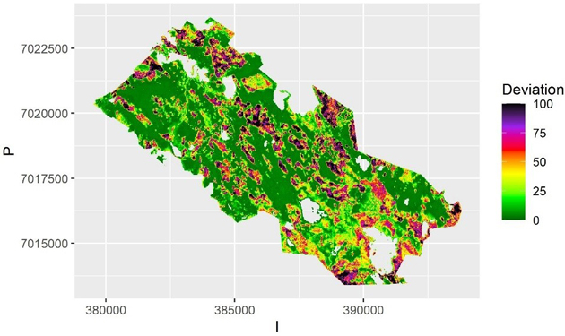
Fig. 4. The average deviation from predicted value of volume over the samples for each pixel using Quantile Random Forest algorithm. The deviation is calculated as half of the interval between the 2.5% and 97.5% quantiles. The scale is truncated at value 100 m3.
The prediction intervals of QRF based on the 2.5% and 97.5% quantiles included on average 82.3% of all the observations in the grid among the 100 simulations assuming independent errors. Thus, the within-sample ensemble-based quantiles underestimated the total uncertainty slightly. With autocorrelated errors the respective values were 81.2 for case b and 82.2 for case c. Thus, introducing autocorrelation did not result in more serious underestimation of uncertainty. The relative RMSE of the mean of the 100 simulated median predictions was 25.8% for independent errors, 28.6 for case b and 25.9 for case c. In repeated simulations, the average coverage of the prediction interval varied from 81.17–82.49.
The map of the mean of the 100 kriging maps is shown in Fig. 5a, and the map of the pixel-level relative standard deviation of these predictions (the between-sample error of a mean prediction) within each pixel is shown in Fig. 5b. This shows the variation due to model selection and parameter estimation. This variation is due to selecting the best three predictors (rather than all) from among all the 17 possible predictors in each simulation. There is still variation between the possible models, but on average less than with the QRF method. Thus, the model selection error is likely underestimated, and the between-sample error in this case depicts mostly the parameter estimation uncertainty. The average relative within-sample variation (Fig. 6) is dominated by residual variation, which was homogeneous for the log-linear model used. It also includes the parameter estimation errors, but not the variation due to model selection.
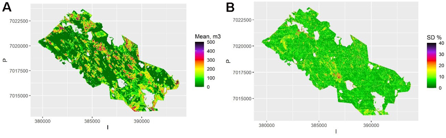
Fig. 5. A) The mean volume prediction for each pixel averaged over the samples using kriging. The scale is truncated at value 500 m3. B) The relative between-sample standard error based on kriging. The scale is truncated at value 40%. View larger in new window/tab.
Fig. 6. The relative within-sample standard error of volume predictions for each pixel based on kriging and averaged over the samples. The scale is truncated at value 40%.
For kriging, the 95% prediction intervals based on within-sample variation for the linear model included 96.3% of all the observations in the grid on average. Thus, the within-sample prediction errors with linear model were very good estimate of the total uncertainty, even though the within-sample variation does not include model selection error. This is likely because the true model was also a log-linear model, and thus the true effect of model selection error in a more complicated case may be underestimated. Moreover, all predictors of the superpopulation model were available, and the sample was representative of the population. The visualization of the uncertainty using the deviation from the expected value is shown in Fig. 7. The within-sample prediction intervals included 96.4% of observations in case b on average and 95.6% in case c. The relative RMSE was 24.86% for the case of independent errors, meaning the linear model was quite similar to QRF with respect to accuracy. For case b the relative RMSE was 26.46% and for case c 24.52%, meaning that the autocorrelation between the prediction errors had a minor effect. In repeated simulations, the coverage of the prediction interval varied from 94.6–96.6.
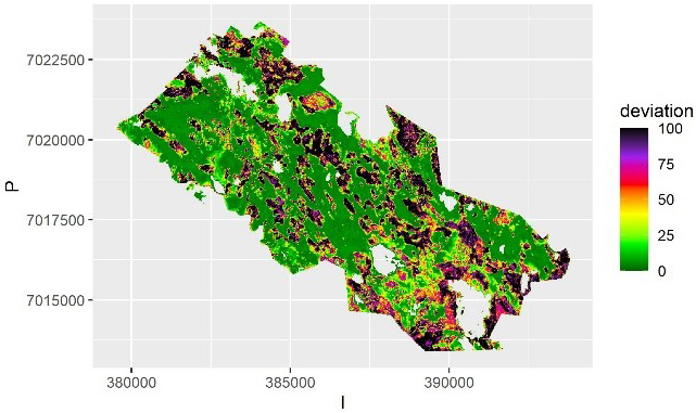
Fig. 7. The average deviation from the predicted value of volume in each pixel over the samples using kriging. The deviation is calculated as half of the prediction interval. The scale is truncated at value 100 m3.
6 Discussion
Maps are commonly used in supporting decision making, as a map is easily comprehensible data. Nevertheless, the wall-to-wall nature of such presentation may give a misleading impression of a high-quality information to a non-professional user. Since the number of maps introducing heavy criticism and comparisons of maps showing coarse errors in the map is large, it can be argued that users of maps do not properly understand the nature of thematic maps as a set of localized model predictions. It can be asked if a thematic map is perceived as more accurate than a set of model predictions, as the thematic maps are compared to the geographical maps rather than model predictions. A map of expected values could give the users a false impression of precision (Grêt-Regamey et al. 2013; Meyer and Pebesma 2022). As a result, most people (even researchers) who need maps use the maps as if they were true values, and ignore the uncertainties.
It is possible that the map uncertainty is not acknowledged when the maps are used, as the means to address and visualize it in a comprehensible way have been lacking (Meyer and Pebesma 2022). Comprehensible way to provide the information of both the mean and variation in the same figure for continuous variables are largely missing. Published tools are found mostly for classified values, but it would be valuable to have suitable tools also for continuous data.
The accuracy assessment protocols used with map products do not clearly inform on if a map is useful for a given purpose or not (Ayanu et al. 2012; McRoberts 2011; Pagella and Sinclair 2014). Meyer and Pebesma (2022) go as far as saying that “showing predicted values on global maps without reliable indication of global and local prediction errors or the limits of the area of applicability, and distributing these for reuse, is not congruent with basic scientific integrity”.
Based on this study, the model ensemble approach with QRF worked reasonably well in depicting the map uncertainty. In this context, by reasonable we mean that using the uncertainty estimate like this will improve decision making and understanding of uncertainties. It is good to remember, however, that if the produced prediction interval is too narrow, it is likely to decrease the quality of decisions rather than improve them. The slight underestimation can be assumed to reflect the relatively large between-sample variation (Fig. 3a versus Fig. 4a): the ensemble (or forest) of regression trees was not able to depict all the variation due to model selection.
The analytical kriging based on a log-linear model provided on average very good prediction intervals from just a single sample. In our example case both the true model and the models estimated from the samples were log-linear models, which probably had an effect. The deviation, or half of the width of a prediction interval seems promising in a sense it can be assumed to be understandable also for the users of the data.
Overall, it seems reasonable to increase the use of kriging in the mapping in the future. A mixed model, assuming a constant correlation between the residual errors within a stand or a plot is commonly utilized in forest inventory. If information of e.g. heights of one or more trees within a stand is measured, the resulting correlation in a case of one random effect,  can be utilized to reduce prediction variance of the heights of other trees with an EBLUP approach (Mehtätalo et al. 2015). Accounting for the autocorrelation in the pixel- or plot-level residual errors using kriging in mapping is essentially similar than using an EBLUP approach in prediction and could be utilized more often also in mapping the forest resources.
Each pixel in a map is a model prediction for a single unit, and inferences regarding the uncertainty for this single pixel are also model-based inferences. However, the term “model-based inference” is typically used in a context of addressing sampling uncertainty in area- or domain-level and using a linear or linearized regression model. The usability of RF or QRF in mapping forest resources and making observation-level inferences is evident. Yet, their usefulness in population-level or domain-level model-based inference is not as evident, as the means to address the uncertainties in these modelling frameworks is very different from the parametric regression models. The same caveat also applies to other types of non-parametric modelling. More studies are needed to assess their usefulness in that context, for instance with utilizing simulation approach rather than analytical formulas.
In this study, the uncertainties concern pixel-level predictions, and can serve in depicting, for instance, areas where the true value can deviate much from the predicted one. However, it is likely that we would need to have uncertainty estimates also for landscape metrics, such as connectivity, mean habitat patch size or similar. In the Gaussian case, the pixel-level kriging variance has an analytical solution. However, for most landscape metrics no analytical solutions exists, but the sequential Gaussian simulation can provide a way to quantify uncertainties also in this case. The simulation-based approach is also available for non-Gaussian models.
Another important potential application is locating areas with required resources, such as areas having at least a required volume. Users of the maps may also wish to pinpoint the proportion of area with a large deadwood volume, or the best quantile of forests regarding for instance the tree species richness. Normal sampling-based inventory does not provide easy estimators for such population parameters. The plot size used in forest inventory is fairly small, and the between-plot or between-pixel variation of volume or dead-wood volume therefore much larger than it is for an aggregation of plots or pixels that constitute one hectare in a forest. Therefore, the quantiles and proportions calculated from the sample data directly are biased, unless the spatial autocorrelation is accounted for in the analysis (Magnussen et al. 2016). Therefore, it is possible that kriging-type approach is a useful method in addressing the proportions and quantiles (Bolin and Lindgren 2015).
In this study, we only discussed the uncertainty analysis only for one variable, which in our simulation experiment was the growing stock volume. Decision making regarding the ecosystem services means, however, making tradeoffs between services. In such a case a joint distribution of the uncertainties will also be needed. Joint distributions of pixel-level uncertainties can be addressed analytically, but for more complicated target variables such as landscape structure metrics, simulation will highly likely be needed. These aspects remain to be studied in the future.
7 Conclusions
The common disputes regarding the quality of forest resources maps point to a lack of proper uncertainty assessments for the maps but also deficiency in the interpretation and use of these maps. There are valid methods available for estimating the uncertainty of the map at each pixel, and also for estimating the uncertainty of more complex landscape features. Kriging especially shows great potential in this respect, but also QRF can be assumed as useful for the users. These methods should be applied more often in published maps. On the other hand, we are lacking suitable methods for visualizing the uncertainties simultaneously with the predictions, and development of such methods for often used GIS systems and spatial statistics packages would be a benefit.
Declaration of openness of research materials, data, and code
The codes and the modelling data are available from the corresponding author with request.
Authors’ contributions
AK did the statistical analysis and the first draft, and MM and LM commented and revised the text.
Funding
The research leading to these results has received funding from the European Union Horizon Europe (HORIZON) Research and Innovation programme under the Grant Agreement no. 101056907 and Academy of Finland flagship programme, the Forest-Human-Machine Interplay (UNITE) flagship [grant numbers 337655 and 357909].
References
Astrup R, Rahlf J, Bjørkelo K, Debella-Gilo M, Gjertsen AK, Breidenbach J (2019) Forest information at multiple scales: development, evaluation and application of the Norwegian forest resources map SR16. Scand J For Res 34: 484–496. https://doi.org/10.1080/02827581.2019.1588989.
Ayanu YZ, Conrad C, Nauss T, Wegmann M, Koellner T (2012) Quantifying and mapping ecosystem services supplies and demands: a review of remote sensing applications. Environm Sci 46: 8529–8541. https://doi.org/10.1021/es300157u.
Baccini A, Laporte N, Goetz S J, Sun M, Dong H (2008) A first map of tropical Africa’s above-ground biomass derived from satellite imagery Environ Res Lett 3, article id 045011. https://doi.org/10.1088/1748-9326/3/4/045011.
Baccini A, Goetz S, Walker W, Laporte NT, Sun M, Sulla-Menashe D, Hacler J, Beck PSA, Dubayah R, Friedl MA, Samanta S, Houghton RA (2012) Estimated carbon dioxide emissions from tropical deforestation improved by carbon-density maps. Nature Clim Change 2: 182–185. https://doi.org/10.1038/nclimate1354.
Balasz A, Liski E, Tuominen S, Kangas A (2022) Comparison of neural networks and k-nearest neighbors methods in forest stand variable estimation using airborne laser data. ISPRS J Photogramm Remote Sens 4, article id 100012. https://doi.org/10.1016/j.ophoto.2022.100012.
Bolin D, Lindgren F (2015) Excursion and contour uncertainty regions for latent Gaussian models. J R Stat Soc Series B Stat Methodol 77: 85–106. https://doi.org/10.1111/rssb.12055.
Breidenbach J, McRoberts RE, Astrup R (2016) Empirical coverage of model-based variance estimators for remote sensing assisted estimation of stand-level timber volume. Remote Sens Environ 173: 274–281. https://doi.org/10.1016/j.rse.2015.07.026.
Breidenbach J, Ellison D, Petersson H, Korhonen KT, Henttonen HM, Wallerman J, Fridman J, Gobakken T, Astrup R, Næsset E (2022) Harvested area did not increase abruptly – how advancements in satellite-based mapping led to erroneous conclusions. Ann For Sci 79, article id 2. https://doi.org/10.1186/s13595-022-01120-4.
Breiman L (2001) Random forests. Mach Learn 45: 5–32. https://doi.org/10.1023/A:1010933404324.
Bugmann H, Seidl R (2022) The evolution, complexity and diversity of models of long-term forest dynamics. J Ecol 110: 2288–2307. https://doi.org/10.1111/1365-2745.13989.
Burkhard B, Kroll F, Nedkov S, Müller F (2012) Mapping ecosystem service supply, demand and budgets. Ecol Indic 21: 17–29. https://doi.org/10.1016/j.ecolind.2011.06.019.
Ceccherini G, Duveiller G, Grassi G, Lemoine G, Avitabile V, Pilli R, Cescatti A (2020) Abrupt increase in harvested forest area over Europe after 2015. Nature 583: 72–77. https://doi.org/10.1038/s41586-020-2438-y.
Ceccherini G, Duveiller G, Grassi G, Lemoine G, Avitabile V, Pilli R, Cescatti A (2022) Potentials and limitations of NFIs and remote sensing in the assessment of harvest rates: a reply to Breidenbach et al. Annals of Forest Science 79, article id 31. https://doi.org/10.1186/s13595-022-01150-y.
Chiles J, Delfiner P (1999) Geostatistics: modeling spatial uncertainty. Wiley, New York. https://doi.org/10.1002/9780470316993.
Christensen R (2011) Plane answers to complex questions: the theory of linear models. Springer, New York. https://doi.org/10.1007/978-1-4419-9816-3.
Efron B, Tibshirani RJ (1998) An introduction to the boostrap. Monographs on Statistics and Applied Probability 57. Chapman and Hall/CRC.
Eigenbrod F, Armsworth PR, Anderson BJ, Heinemeyer A, Gillings S, Roy DB, Thomas CD, Gaston KJ (2010) The impact of proxy-based methods on mapping the distribution of ecosystem services. Journal of Applied Ecology 47: 377–385. https://doi.org/10.1111/j.1365-2664.2010.01777.x.
Esteban J, McRoberts RE, Fernández-Landa A, Tomé JL, Nӕsset E (2019) Estimating forest volume and biomass and their changes using random forests and remotely sensed data. Remote Sens 11, article id 1944. https://doi.org/10.3390/rs11161944.
Fouedjio F, Klump J (2019) Exploring prediction uncertainty of spatial data in geostatistical and machine learning approaches. Environ Earth Sci 78, article id 38. https://doi.org/10.1007/s12665-018-8032-z.
Freeman EA, Moisen GG (2015) An application of quantile random forests for predictive mapping of forest attributes. In: Stanton SM, Christensen GA. Pushing boundaries: new directions in inventory techniques and applications: forest Inventory and Analysis (FIA) symposium 2015. PNW-GTR-931, Department of Agriculture, Forest Service, Pacific Northwest Research Station, Portland, OR, U.S. https://doi.org/10.2737/PNW-GTR-931.
Gelman A, Carlin JB, Stern HS, Dunson DB, Vehtari A, Rubin DB (2013) Bayesian data analysis, third edition. CRC Press. https://doi.org/10.1201/b16018.
Goovaerts P (2001) Geostatistical modelling of uncertainty in soil science. Geoderma 103: 3–26. https://doi.org/10.1016/S0016-7061(01)00067-2.
Gräler B, Pebesma E (2011) The pair-copula construction for spatial data: a new approach to model spatial dependency. Procedia Environ Sci 7: 206–211. https://doi.org/10.1016/j.proenv.2011.07.036.
Gregoire TG (1998) Design-based and model-based inference in survey sampling: appreciating the difference. Can J For Res 28: 1429–1447. https://doi.org/10.1139/x98-166.
Grêt-Regamey A, Brunner SH, Altwegg J, Bebi P (2013) Facing uncertainty in ecosystem services-based resource management. J Environ Manage 127: 145–154. https://doi.org/10.1016/j.jenvman.2012.07.028.
Hansen MC, Potapov PV, Moore R, Hancher M, Turubanova SA,Tyukavina A, Thau D, Stehman SV, Goetz SJ, Loveland TR, Kommareddy A, Egorov A, Chini L, Justice CO, Townshend JRG (2013) High-resolution global maps of 21st-century forest cover change. Science 342: 850–853. https://doi.org/10.1126/science.1244693.
Hauglin M, Rahlf J, Schumacher J, Astrup R, Breidenbach J (2021). Large scale mapping of forest attributes using heterogeneous sets of airborne laser scanning and National Forest Inventory data. For Ecosyst 8, article id 65. https://doi.org/10.1186/s40663-021-00338-4.
Hengl T, Heuvelink GBM, Rossiter DG (2007) About regression-kriging: from equations to case studies. Comput Geosci 33: 1301–1315. https://doi.org/10.1016/j.cageo.2007.05.001.
Journel AG (1996) Modelling uncertainty and spatial dependence: stochastic imaging. Int J Geogr Inf Syst 10: 517–522. https://doi.org/10.1080/02693799608902094.
Kangas A (1998) Effect of errors-in-variables on coefficients of a growth model and on prediction of growth. For Ecol Manag 102: 203–212. https://doi.org/10.1016/S0378-1127(97)00161-8.
Kangas A, Mehtätalo L (2021) Monimuotoisuuskartta kaipaa korjaamista. Metsätieteen Aikakauskirja, article id 10625. https://doi.org/10.14214/ma.10625.
Kangas A, Heikkinen E, Maltamo M (2004) Accuracy of partially visually assessed stand characteristics – a case study of Finnish inventory by compartments. Can J For Res 34: 916–930. https://doi.org/10.1139/x03-266.
Kangas A, Astrup R, Breidenbach J, Fridman J, Gobakken T, Korhonen KT. Maltamo M, Nilsson M, Nord-Larsen T, Næsset E, Olsson H (2018) Remote sensing and forest inventories in Nordic countries – roadmap for the future. Scand J Forest Res 33: 397–412. https://doi.org/10.1080/02827581.2017.1416666.
Kangas A, Räty M, Korhonen KT, Vauhkonen J, Packalen T (2019) Catering information needs from global to local scales – potential and challenges with national forest inventories. Forests 10, article id 800. https://doi.org/10.3390/f10090800.
Kasraei B, Heung B, Saurette DD, Schmidt MG, Bulmer CE, Bethel W (2021) Quantile regression as a generic approach for estimating uncertainty of digital soil maps produced from machine-learning. Environ Model Softw 144, article id 105139. https://doi.org/10.1016/j.envsoft.2021.105139.
Katila M, Rajala T, Kangas A (2020) Assessing local trends in indicators of ecosystem services with a time series of forest resource maps. Silva Fenn 54, article id 10347. https://doi.org/10.14214/sf.10347.
Kaye N, Hartley A, Hemming D (2012) Mapping the climate: guidance on appropriate techniques to map climate variables and their uncertainty. Geosci Model Dev 4: 245–256. https://doi.org/10.5194/gmd-5-245-2012.
Kotivuori E, Kukkonen M, Mehtätalo L, Maltamo M, Korhonen L, Packalen P (2020) Forest inventories for small areas using drone imagery without in-situ field measurements. Remote Sens Environ 237, article id 111404. https://doi.org/10.1016/j.rse.2019.111404.
Lier M, Köhl M, Korhonen KT, Linser S, Prins K (2021) Forest relevant targets in EU policy instruments – can progress be measured by the pan-European criteria and indicators for sustainable forest management? For. Policy Econ 128, article id 102481. https://doi.org/10.1016/j.forpol.2021.102481.
Maes J, Egoh B, Willemen L, Liquete C, Vihervaara P, Schägner JP, Grizzetti B, Drakou EG, LaNotte A, Zulian G, Bouraoui F, Paracchini ML, Braat L, Bidoglio G (2012) Mapping ecosystem services for policy support and decision making in the European Union. Ecosyst Serv 1: 31–39. https://doi.org/10.1016/j.ecoser.2012.06.004.
Magnussen S, Breidenbach J (2017) Model-dependent forest stand-level inference with and without estimates of stand-effects. Forestry 90: 675–685. https://doi.org/10.1093/forestry/cpx023.
Magnussen S, Fehrmann L (2019) In search of a variance estimator for systematic sampling. Scand J Forest Res 34: 300–312. https://doi.org/10.1080/02827581.2019.1599063.
Magnussen S, Mandallaz D, Lanz A, Ginzler C, Næsset E, Gobakken T (2016) Scale effects in survey estimates of proportions and quantiles of per unit area attributes. For Ecol Manag 364: 122–129. https://doi.org/10.1016/j.foreco.2016.01.013.
McRoberts RE (2011) Satellite image-based maps: scientific inference or pretty pictures? Remote Sens Environ 115: 715–724. https://doi.org/10.1016/j.rse.2010.10.013.
Mehtätalo L, Lappi J (2020) Biometry for forestry and environmental data. CRC Press, New York. https://doi.org/10.1201/9780429173462.
Meinshausen N (2006) Quantile regression forests. J Mach Learn Res 7: 983–999.
Meinshausen N (2017) quantregForest: quantile regression forests. R package version 1.3-7. https://CRAN.R-project.org/package=quantregForest.
Meyer H, Pebesma E (2021) Predicting into unknown space? Estimating the area of applicability of spatial prediction models. Methods Ecol Evol 12: 1620–1633. https://doi.org/10.1111/2041-210X.13650.
Meyer H, Pebesma E (2022) Machine learning-based global maps of ecological variables and the challenge of assessing them. Nat Commun 13, article id 2208. https://doi.org/10.1038/s41467-022-29838-9.
Mikkonen N, Leikola N, Lahtinen A, Lehtomäki J, Halme P (2018) Monimuotoisuudelle tärkeät metsäalueet Suomessa. Puustoisten elinympäristöjen monimuotoisuusarvojen Zonation -analyysien loppuraportti. Suomen ympäristökeskuksen raportteja 9/2018. http://hdl.handle.net/10138/234359.
Mikkonen N, Leikola N, Halme P, Heinaro E, Lahtinen A, Tanhuanpää T (2019) Modeling of dead wood potential based on tree stand data. Forests 11, article id 913. https://doi.org/10.3390/f11090913.
Mitchard ETA, Saatchi SS, Lewis SL, Feldpausch TR, Gerard FF, Woodhouse IH, Meir P (2011) Comment on a first map of tropical Africa’s above-ground biomass derived from satellite imagery. Environ Res Lett 6, article id 049001. https://doi.org/10.1088/1748-9326/6/4/049001.
Mitchard ET, Saatchi SS, Baccini A, Asner GP, Goetz SP, Harris NL, Brown S (2013) Uncertainty in the spatial distribution of tropical forest biomass: a comparison of pan-tropical maps. Carbon Balance Manage 8, article id 10. https://doi.org/10.1186/1750-0680-8-10.
Mu W, Tong D (2019) Choropleth mapping with uncertainty: a maximum likelihood–based classification scheme. Ann Am Assoc Geogr 109: 1493–1510. https://doi.org/10.1080/24694452.2018.1549971.
Nilsson M, Nordkvist K, Jonzén J, Lindgren N, Axensten P, Wallerman J, Egberth M, Larsson S, Nilsson L, Eriksson J, Olsson H (2017) A nationwide forest attribute map of Sweden predicted using airborne laser scanning data and field data from the National Forest Inventory. Remote Sens Environ 194: 447–454. https://doi.org/10.1016/j.rse.2016.10.022.
Nisbet R, Elder J, Miner G (2009) Handbook of statistical analysis and data mining applications. Academic Press. https://doi.org/10.1016/B978-0-12-374765-5.X0001-0.
Nord-Larsen T, Riis-Nielsen T, Ottosen MB (2017) Forest resource map of Denmark: mapping of Danish forest resource using ALS from 2014–2015. IGN Report, Department of Geosciences and Natural Resource Management, University of Copenhagen.
Olofsson P, Foody GM, Herold M, Stehman SV, Woodcock CE, Wulder MA (2014) Good practices for estimating area and assessing accuracy of land change. Remote Sens Environ 148: 42–57. https://doi.org/10.1016/j.rse.2014.02.015.
Ojanen M, Brockhaus M, Korhonen-Kurki K, Petrokofsky G (2021) Navigating the science-policy interface: forest researcher perspectives. Environ Sci Policy 118: 10–17. https://doi.org/10.1016/j.envsci.2021.01.002.
Pagella TF, Sinclair FI (2014) Development and use of typology of mapping tools to assess their fitness for supporting management of ecosystem service provision. Landsc Ecol 29: 383–399. https://doi.org/10.1007/s10980-013-9983-9.
Palahi M, Valbuena R, Senf C, Acil N, Pugh TAM, Sadler J, Seidl R, Potapov P, Gardiner B, Hetemäki L, Chirici G, Francini S, Hlásny T, Lerink BJM, Olsson H, Olabarria JRG, Ascoli D, Asikainen A, Bauhus J, Berndes G, Donis J, Fridman J, Hanewinkel M, Jactel H, Lindner M, Marchetti M, Marušák R, Sheil D, Tomé M, Trasobares A, Verkerk PJ, Korhonen M, Nabuurs GJ (2021) Concerns about reported harvests in European forests. Nature 592: E15–E17. https://doi.org/10.1038/s41586-021-03292-x.
Pebesma EJ (2004) Multivariable geostatistics in S: the gstat package. Comput Geosci 30: 683–691. https://doi.org/10.1016/j.cageo.2004.03.012.
Peters J, Verhoest NEC, Samson R, Van Meirvenne M, Cockx L, De Baets B (2009) Uncertainty propagation in vegetation distribution models based on ensemble classifiers. Ecol Modell 220: 791–804. https://doi.org/10.1016/j.ecolmodel.2008.12.022.
Piironen J, Vehtari A (2017) Comparison of Bayesian predictive methods for model selection. Stat Comput27: 711–735. https://doi.org/10.1007/s11222-016-9649-y.
Plant R (2019) Spatial data analysis in ecology and agriculture using R, 2nd edition. CRC press, Boca Raton. https://doi.org/10.1201/9781351189910.
Retchless DP, Brewer CA (2016) Guidance for representing uncertainty on global temperature change maps. Int J Climatol 36: 1143–1159. https://doi.org/10.1002/joc.4408.
Saarela S, Schnell S, Tuominen S, Balázs A, Hyyppä J, Grafström A, Ståhl G (2016) Effects of positional errors in model-assisted and model-based estimation of growing stock volume. Remote Sens Environ 172: 101–108 https://doi.org/10.1016/j.rse.2015.11.002.
Saarela S, Wästlund A, Holmström E, Mensah AA, Holm S, Nilsson M, Fridman J, Ståhl G (2020) Mapping aboveground biomass and its prediction uncertainty using LiDAR and field data, accounting for tree-level allometric and LiDAR model errors. For Ecosyst 7, article id 43. https://doi.org/10.1186/s40663-020-00245-0.
Saatchi SS, Harris NL, Brown S, Lefsky M, Mitchard ETA, Salas W, Zutta BR, Buermann W, Lewis SL, Hagen S, Petrova S, White L, Silman M, Morel A (2011) Benchmark map of forest carbon stocks in tropicalregions across three continents. PNAS 108: 9899–9904. https://doi.org/10.1073/pnas.1019576108.
Sagar A, Vega C, Bouriaud O, Piedallu C, Renaud JP (2022) Multisource forest inventories: a model-based approach using k-NN to reconcile forest attributes statistics and map products. ISPRS J Photogramm Remote Sens 192: 175–188. https://doi.org/10.1016/j.isprsjprs.2022.08.016.
Schabenberger O, Gotway CA (2005) Statistical methods for spatial data analysis. Chapman and Hall/CRC, New York. https://doi.org/10.1201/9781315275086.
Schulp CJE, Burkhard B, Maes J, Van Vliet J, Verburg PH (2014) Uncertainties in ecosystem service maps: a comparison on the European scale. PloS ONE 9, article id e109643. https://doi.org/10.1371/journal.pone.0109643.
Seber GAF, Wild CJ (1989) Nonlinear regression. John Wiley and Sons. https://doi.org/10.1002/0471725315.
Szatmári G, Pásztor L (2019) Comparison of various uncertainty modelling approaches based on geostatistics and machine learning algorithms. Geoderma 337: 1329–1340. https://doi.org/10.1016/j.geoderma.2018.09.008.
Tomppo E (1996) Multi-source National Forest Inventory of Finland. New thrusts in forest inventory. Proceedings of the Subject Group S4.02–00 ‘Forest Resource Inventory and Monitoring’ and Subject Group S4.12– 00 ‘Remote Sensing Technology’. Vol. I. IUFRO XX World Congress, 6–12 August 1995, Tampere, Finland. European Forest Institute EFI Proceedings No. 7. ISBN 952-9844-15-8.
Tuominen S, Pitkänen T, Balázs A, Kangas A (2017) Improving Multi-Source National Forest Inventory by 3D aerial imaging. Silva Fenn 51, article id 7743. https://doi.org/10.14214/sf.7743.
Vaysse K, Lagacherie P (2017) Using quantile regression forest to estimate uncertainty of digital soil mapping products. Geoderma 291: 55–64. https://doi.org/10.1016/j.geoderma.2016.12.017.
Wernick IK, Ciais P, Fridman J, Högberg P, Korhonen KT, Nordin A, Kauppi PE (2021) Quantifying forest change in the European Union. Nature 592: E13–E14. https://doi.org/10.1038/s41586-021-03293-w.
Zhang Y, Liang S, Yang L (2019) A review of regional and global gridded forest biomass datasets. Remote Sens 11, article id 2744. https://doi.org/10.3390/rs11232744.
Total of 79 references.
Send to email
