Tuomas Yrttimaa  ,
Lauri Liikonen,
Aapo Erkkilä,
Mikko Vastaranta
,
Lauri Liikonen,
Aapo Erkkilä,
Mikko Vastaranta
Terrestrial laser scanning point clouds and tree attributes from 55 sample plots at the Evo test site (spring 2024)
Yrttimaa T., Liikonen L., Erkkilä A., Vastaranta M. (2025). Terrestrial laser scanning point clouds and tree attributes from 55 sample plots at the Evo test site (spring 2024). Silva Fennica vol. 59 no. 1 article id 24066. https://doi.org/10.14214/sf.24066
Highlights
- Terrestrial laser scanning dataset from 55 sample plots (32 × 32 m) representing boreal forests of Southern Finland
- Data was acquired in April–May 2024 using a Riegl VZ-400i scanner, providing multiple returns per pulse
- Each point is annotated with reflectance, return properties, and tree linkage
- Crown and stem diameters were derived for further analysis, advancing tree and forest research applications.
Abstract
Terrestrial laser scanning (TLS) is an active remote sensing technique that digitizes trees and forest stands by capturing range measurements, resulting in detailed point clouds. To support the development of computational methods for tree and forest stand characterization, as well as to facilitate the exploration of tree structures, we collected TLS data from 55 sample plots (32 m × 32 m) and 6320 trees in Evo, Southern Finland. Data acquisition was conducted during April–May 2024 using a Riegl VZ-400i terrestrial laser scanner (Riegl Laser Measurement Systems GmbH, Austria), capable of recording up to eight returns per laser pulse. This dataset includes TLS point clouds in the projected coordinate reference system commonly used in Finland (ETRS-TM35FIN). Each point is annotated with reflectance, return number, return count, and height above ground. Additionally, information linking each return to its originating tree is provided. For individual trees, the point clouds were further processed to derive key attributes such as crown projection area, crown diameter, and stem diameter. In addition, tree species was derived by linking the TLS-based tree measurements with field inventory data. Here, we describe and share these curated TLS data files and related tree measurements, which offer a valuable resource for advancing tree- and forest-related research and applications.
Keywords
boreal forest;
ground-based LiDAR;
LIS TreeAnalyzer;
point cloud processing;
Riegl VZ-400i;
tree characterization;
tree reconstruction
-
Yrttimaa,
School of Forest Sciences, University of Eastern Finland, FI-80101 Joensuu, Finland
 https://orcid.org/0000-0003-2648-523X
E-mail
tuomas.yrttimaa@uef.fi
https://orcid.org/0000-0003-2648-523X
E-mail
tuomas.yrttimaa@uef.fi
- Liikonen, School of Forest Sciences, University of Eastern Finland, FI-80101 Joensuu, Finland E-mail lauriliik@uef.fi
- Erkkilä, School of Forest Sciences, University of Eastern Finland, FI-80101 Joensuu, Finland E-mail aapo.erkkila@uef.fi
-
Vastaranta,
School of Forest Sciences, University of Eastern Finland, FI-80101 Joensuu, Finland
https://orcid.org/0000-0001-6552-9122
E-mail
mikko.vastaranta@uef.fi
Received 22 November 2024 Accepted 3 May 2025 Published 8 May 2025
Views 19730
Available at https://doi.org/10.14214/sf.24066 | Download PDF

Supplementary Files
1 Introduction
Terrestrial laser scanning (TLS) has enabled researchers and practitioners to collect detailed point cloud data characterizing trees and stands. This active remote sensing technique digitizes objects of interest through range measurements, resulting in point clouds (x, y, and z coordinates representing reflections from objects). TLS has been used in forest mensuration research for approximately 20 years (Liang et al. 2016; Calders et al. 2020). From the early days, the technology demonstrated its power in mapping vegetation structures and trees, particularly in measuring attributes such as location, stem dimensions at multiple heights, and crown properties (Calders et al. 2020). These attributes were often excluded from field surveys due to the lack of efficient measurement methodologies (Liang et al. 2016). The widespread adoption of TLS in forest measurement was hindered by the high costs of the sensors, the lack of algorithms and software, and insufficient general knowledge on how to collect and process the data (Fassnacht et al. 2024). Moreover, the expensive equipment was not always well-suited to varying conditions in the field. It should be also noted that for the basic suite of tree and stand attributes, traditional tools like calipers and clinometers often provided more reliable measurements (Luoma et al. 2017; Liang et al. 2018).
The use of TLS in forest mensuration research and forest research in general has increased significantly. Several research groups are utilizing scanners to measure individual trees and sample plots (Liang et al. 2018; Calders et al. 2020; Fassnacht et al. 2024). Additionally, numerous organizations conducting forest inventories for forest management and planning are increasingly interested in TLS measurements. To enable researchers, but also research, development and innovation professionals to utilize TLS data and understand how it can be used to measure trees and forests, we have collected TLS data from forest monitoring plots distributed around the Evo research area. Subsequently, we have georeferenced the scans to allow users to integrate them with other geospatial datasets. In addition, we have segmented to the georeferenced TLS point clouds, individual trees from the point clouds and determined their location, stem diameter, height, and crown characteristics using commercial software. This allows users to utilize either the collected point clouds from sample plots or the interpreted tree attributes for their research and development purposes.
2 Methods
2.1 Study area and selection of the sample plots
The data collection was conducted at the Evo study site, located in Southern Finland (61°12´N, 25°07´E). The site encompasses typical southern boreal forest conditions, ranging from single-species to mixed-species stands, and from even-aged to multi-layered structures. Scots pine (Pinus sylvestris L.), Norway spruce (Picea abies (L.) H. Karst.), birches (Betula L. spp.), and European aspen (Populus tremula L.) are the main tree species. TLS point clouds were collected from 55 sample plots (32 m × 32 m) to reconstruct the 3D architecture of individual trees across various growing conditions and development phases. The sample plots represent a range of canopy heights and closures in Evo, forming a representative sample of regularly monitored plots initially established in 2014 (see the sampling description in Yu et al. 2015). As such, they encompass diverse forest structures.
2.2 Measurements
TLS measurements were carried out under leaf-off conditions between April 22 and May 14, 2024, using a Riegl VZ-400i (Riegl Laser Measurement Systems GmbH, Austria) time-of-flight terrestrial laser scanner (Table 1). We generated hemispherical point clouds by combining two different scanning configurations. In the scanner’s standard upright configuration, it provides a 100° vertical and 360° horizontal field of view. To achieve a full field of view, we used a tilt-mount between the scanner and the tripod, enabling the scanner to be rotated 90° from its upright orientation. This setup resulted in a 360° vertical and 100° horizontal field of view in the tilted position. Each plot was scanned from nine different locations (scan positions) arranged evenly around the sample plot, spaced approximately 16 m apart to ensure comprehensive coverage of the plot area. Upright scans were conducted at all nine locations, while tilted scans were performed at alternating positions (Fig. 1). One to three additional scan positions were added for plots 1013, 1014, 1016, 1031, 1037, 1041, 1055, 1057, 1089, 1092, 1112, 1120, 1132, 2028, and 2113, to account for vegetation complexity or challenging topography. During data acquisition, the scanner employed integrated global navigation satellite system (GNSS) and inertial measurement unit (IMU) sensors to estimate its position and orientation in real time. This functionality enabled on-board co-registration of scans without requiring external reference targets.
| Table 1. Terrestrial laser scanning data acquisition parameters. | |
| Parameter | Details |
| Acquisition Dates | 22 April – 14 May 2024 |
| Conditions | Leaf-off |
| Scanner Model | Riegl VZ-400i |
| Measurement principle | Time-of-flight |
| Wavelength | 1550 nm |
| Laser Beam Diameter (at exit) | 7 mm |
| Beam Divergence | 0.35 mrad (at the 1/e² points) |
| Beam Diameter at 10, 20 and 30 m | 10, 14, 18 mm |
| Pulse Repetition Rate | 600 kHz |
| Maximum Returns per Pulse | Up to 8 |
| Scan Pattern | ‘Panorama 40’ |
| Angular Resolution | 0.04° |
| Point Spacing at 10 m | 3.5 mm |
| Vertical Field of View | 100° (Scan Position, upright), 360° (Scanner tilted 90°) |
| Horizontal Field of View | 360° (Scan Position, upright), 100° (Scanner tilted 90°) |
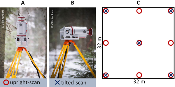
Fig. 1. Illustration of the applied point cloud data acquisition setup. A Riegl VZ-400i terrestrial laser scanner equipped with a tilt-mount to capture both upright-positioned (A) and tilted scans (B), enabling a combined 360° vertical and horizontal field of view. Nine scan positions were utilized to capture the full extent of the sample plots (C).
2.3 Point clouds from the sample plots, including segmentation by individual trees
The individual scans were co-registered and merged using RiSCAN PRO software (version 2.19.3), provided by the scanner manufacturer. To reduce oversampling of surfaces close to the scanner – such as the ground and lower stem sections – the merged point clouds were thinned using 1-mm voxelization. This decimation did not affect the point density of surfaces farther from the scanner, such as upper tree crowns, where the original density was preserved. The point clouds were delineated considering sample plot borders while preserving a buffer around the plot to include neighboring trees for those located along the plot edges. Individual tree detection and segmentation were carried out using the LIS TreeAnalyzer extension, a plugin within RiSCAN PRO developed by Laserdata GmbH (Innsbruck, Austria; Groiss and Handl 2024). Ground points were first identified following Axelsson’s method (2000), enabling the creation of a digital elevation model. Subsequently, Z-coordinates were normalized to represent height above ground. Tree identification began with the extraction of a horizontal slice of the point cloud, 30 cm thick, where stem cross-sections were expected to form circular patterns. This slicing was conducted between heights of 1.5–2.5 m, depending on sample plot structure and e.g. the presence of understory and branching density.
To enhance detection accuracy, the extracted slice was filtered to exclude points likely originating from branches rather than stems. This was achieved using scanner-derived attributes: Reflectance (distance-corrected laser pulse intensity, measured in dB) and Deviation (a measure of waveform distortion, represented as an integer between 1 and 20). Preliminary experiments indicated that smooth surfaces, such as the stems, exhibited high Reflectance values and low Deviation values. Based on these findings, points with Reflectance < –2.5 dB or Deviation > 3 were filtered out.
The filtered points were assumed to form circular clusters representing stem cross-sections when projected onto the XY plane. A Hough Circle Transform algorithm, following principles described by Illingworth and Kittler (1987), was employed to identify these circular shapes with a minimum separation of 0.1 m. The identified circles were evaluated based on two metrics produced by the LIS TreeAnalyzer plugin: ‘circle completeness’, which assessed the extent of the stem circumference captured, and ‘goodness of fit’, which quantified how well the circle matched the point distribution. These metrics aided manual validation in identifying false positives, such as points representing branches or undergrowth that were mistakenly segmented as trees. Trees missed by the automatic detection process were manually force-identified to ensure all stems were segmented.
The identified tree locations served as seed points for a bottom-up segmentation process, which delineated individual trees, including their stems and branches, within the sample plot point cloud. This segmentation used a 3D Dijkstra Region Growing algorithm, as described by Bremer et al. (2018), to determine the shortest paths from seed points to the top of the canopy. Points connected to the same seed via the shortest path were assigned to the same tree. To address occlusion-related gaps typical in TLS data – especially in the upper crown regions – path discontinuities up to a maximum gap size of 0.6 m were allowed. A minimum height threshold of 1.5 m was also applied to exclude seedlings and low vegetation from segmentation as trees. Points not associated with any identified tree were not omitted but assigned a classification ‘not a tree’ (tree ID = 0).
A total of 6320 trees were segmented from the point clouds, with an average of 115 trees per sample plot, ranging from 30 to 369 trees. Based on the tree segmentation, the following attributes were derived for each tree:
• Stem diameter: Measured by a circle fit into points at the height where the tree was identified.
• Tree height: Calculated as the vertical range of the tree’s point cloud.
• Crown projection area and crown diameter: Determined from the properties of a polygon enveloping the tree point cloud projected onto the XY plane.
• Circle completeness and goodness of fit: Metrics related to the Hough circle detection method used for tree identification. These metrics reflect the reliability of tree identification and diameter measurement (see the description above).
To address the 1–2 m GNSS localization accuracy during data acquisition, the dataset was georeferenced against real-time kinematic GNSS-measured tree maps from the 2014 field inventory (Yu et al. 2015). For each sample plot, correspondences were established between the XY coordinates of TLS-segmented trees and field-measured trees. These matches were used to compute a 2D rigid transformation (XY translation and Z-axis rotation) to spatially align the datasets.
In addition, tree species information was extracted from the 2014 field inventory data for trees where this information was available. It should be noted that species data were not available for: 1) buffer trees located outside the sample plot borders but included in the dataset, and 2) trees that were not measured in 2014 because their diameter did not exceed the 5 cm threshold. The tree species distribution is presented in Table 2.
| Table 2. Data record and their descriptions. ETRS-TM35FIN (EPSG:3067) is a projected coordinate reference system (CRS) commonly used in Finland. N2000 is the used vertical reference system. Tree species distribution is presented for tree attributes. For stand-level forest inventory attributes, the minimum–maximum ranges as well as mean values (in parenthesis) across the sample plots is presented. | |||
| Data record | Description | Data format | |
| Tree-segmented point cloud data | A point cloud file (one per each sample plot) containing the following attributes for each point record: | .laz (version 1.4) | |
| - X coordinate (Easting) [m], ETRS-TM35FIN (epsg: 3067) | |||
| - Y coordinate (Northing) [m], ETRS-TM35FIN (epsg: 3067) | |||
| - Z coordinate (Height) [m], N2000 | |||
| - Reflectance (distance-corrected intensity) [dB] (stored as Extra Field) | |||
| - Return number | |||
| - Number of returns | |||
| - Scan position ID (stored as Point Source ID) | |||
| - Height above ground level [m] (stored as Extra Field ‘h’) | |||
| - Tree ID number (stored as Extra Field ‘treeid’) | |||
| Tree attributes | A text file containing the following attributes for each tree segmented, in the order of their appearance: | .csv (comma delimited) | |
| - x: X coordinate of stem cross section mid-point (Easting) [m], ETRS-TM35FIN (epsg: 3067) | |||
| - y: Y coordinate of stem cross section mid-point (Northing) [m], ETRS-TM35FIN (epsg: 3067) | |||
| - z: Z coordinate of stem cross section height [m], N2000 | |||
| - plot_id: Sample plot ID number | |||
| - tree_id: Tree ID number | |||
| - tree_sp: Tree species: | n | ||
| 0 = not defined | 1882 | ||
| 1 = Scots pine (Pinus sylvestris L.) | 1811 | ||
| 2 = Norway spruce (Picea abies (L.) H. Karst.) | 1415 | ||
| 3 = Birches (Betula L. spp.) | 989 | ||
| 4 = European aspen (Populus tremula L.) | 71 | ||
| 5 = grey alder (Alnus incana (L.) Moench) | 44 | ||
| 6 = common alder (Alnus glutinosa (L.) Gaertn.) | 1 | ||
| 7 = rowan (Sorbus aucuparia L.) | 68 | ||
| 9 = Larix spp. | 1 | ||
| 10 = Fir (Abies spp.) | 6 | ||
| 11 = unknown species | 29 | ||
| 12 = common juniper (Juniperus communis L.) | 3 | ||
| - stem_diam: Stem diameter at the height of tree identification [m] | |||
| - tree_height: Tree height [m] | |||
| - crown_area: Crown projection area [m2] | |||
| - crown_diam: Crown diameter [m] | |||
| - circle_compl: Circle completeness [%] (related to Hough circle finding) | |||
| - goodness_of_fit: Goodness of fit [%] (related to Hough circle finding) | |||
| - pts_on_circle: n.o. points on the fitted circle (related to Hough circle finding) | |||
| - slice_height: point cloud slicing height (± 0.15 m) for tree identification | |||
| Forest inventory attributes | A text file containing stand-level forest inventory attributes for each sample plot, in the order of their appearance in the file: | .csv (comma delimited) | |
| - plot_id: Sample plot ID number | |||
| - x: X coordinate of sample plot center (Easting) [m], ETRS-TM35FIN (epsg: 3067) | |||
| - y: Y coordinate of sample plot center (Northing) [m], ETRS-TM35FIN (epsg: 3067) | |||
| min–max (mean) | |||
| - N: number of trees per hectare | 166–2080 (697) | ||
| - G: mean basal area [m2/ha] | 4.9–50.9 (30.2) | ||
| - V: total stem volume [m3/ha] | 40.9–625.1 (324.0) | ||
| - Dg: basal area-weighted mean diameter [cm] | 16.9–45.2 (28.7) | ||
| - Hg: basal area-weighted mean height [m] | 11.8–31.5 (22.1) | ||
| - Pine_BA%: Scots pine basal area perc. [%] | 0–99.9 (55.5) | ||
| - Spruce_BA%: Norway spruce basal area perc. [%] | 0–100 (26.7) | ||
| - Birch_BA%: Deciduous trees basal area perc. [%] | 0–99.3 (17.8) | ||
Automatic point cloud processing methods (Yrttimaa et al. 2020) were applied to derive stand-level forest inventory attributes from the tree-segmented point clouds. These attributes include the number of trees per hectare, mean basal area, total stem volume, as well as basal area-weighted mean diameter and -height. In addition, basal area proportions for Scots pine, Norway spruce, and deciduous trees were computed based on 2014 field inventory data. These metrics provide context for data users by describing the structural conditions of the sample plots.
4 Technical validation
The relative 3D positioning accuracy of points in the TLS data is 3 mm at 50-m distance, according to the manufacturer’s test protocol. Data georeferencing achieved an absolute localization accuracy of <3 cm when referenced to the 2014 tree maps. Tree identification was manually controlled as an attempt to identify as many trees as possible, yielding 90% overall accuracy when compared against field inventory data that was not, however, inspected for possible missing trees due to harvesting or natural disturbances. It is likely that small trees in the most complex sample plots have remained undetected due to incomplete point cloud reconstruction as typical to TLS-based forest characterization within the study site (Liang et al. 2018; Yrttimaa et al. 2019, 2020).
Usage notes
The data is licensed under a Creative Commons Attribution 4.0 International (CC BY 4.0) license and is openly available at: https://doi.org/10.23729/fd-5a800660-8bd8-35ef-ac9f-ac5c45f7fa77.
Funding
The data acquisition and processing were supported by the Research Council of Finland through funding provided for the Measuring Spatiotemporal Changes in Forest Ecosystem research infrastructure (Scan4est FIRI), grant number 346383, and Forest-Human-Machine Interplay (UNITE) flagship, grant number 357906.
Authors’ contributions
Tuomas Yrttimaa (Conceptualization, Supervision, Methodology, Writing – original draft), Lauri Liikonen (Investigation, Formal analysis, Data curation, Writing – review and editing), Aapo Erkkilä (Investigation, Formal analysis, Data curation, Writing – review and editing), Mikko Vastaranta (Conceptualization, Resources, Funding acquisition, Project management, Writing – original draft).
References
Axelsson P (2000) DEM generation from laser scanner data using adaptive TIN models. Int Arch Photogramm Remote Sens 33(B4): 110–117.
Bremer M, Wichmann V, Rutzinger M (2018) Multi-temporal fine-scale modelling of Larix decidua forest plots using terrestrial LiDAR and hemispherical photographs. Remote Sens Environ 206: 189–204. https://doi.org/10.1016/j.rse.2017.12.023.
Calders K, Adams J, Armston J, Bartholomeus H, Bauwens S, Bentley LP, Chave J, Danson FM, Demol M, Disney M, Gaulton R 2020 Terrestrial laser scanning in forest ecology: expanding the horizon. Remote Sens Environ 251, article id 112102. https://doi.org/10.1016/j.rse.2020.112102.
Fassnacht FE, White JC, Wulder MA, Næsset E 2024. Remote sensing in forestry: current challenges, considerations and directions. Forestry 97: 11–37. https://doi.org/10.1093/forestry/cpad024.
Groiss B, Handl M (2024) Efficient extraction of tree parameters from 3D point clouds. EGU General Assembly 2024, Vienna, Austria, 14–19 Apr, EGU24-9834. https://doi.org/10.5194/egusphere-egu24-9834.
Illingworth J, Kittler J (1987) The Adaptive Hough Transform. IEEE T Pattern Anal 9: 690–698. https://doi.org/10.1109/TPAMI.1987.4767964.
Liang X, Kankare V, Hyyppä J, Wang Y, Kukko A, Haggrén H, Yu X, Kaartinen H, Jaakkola A, Guan F, Holopainen M (2016) Terrestrial laser scanning in forest inventories. ISPRS J Photogramm Remote Sens 115: 63–77. https://doi.org/10.1016/j.isprsjprs.2016.01.006.
Liang X, Hyyppä J, Kaartinen H, Lehtomäki M, Pyörälä J, Pfeifer N, Holopainen M, Brolly G, Francesco P, Hackenberg J, Huang H (2018) International benchmarking of terrestrial laser scanning approaches for forest inventories. ISPRS J Photogramm Remote Sens 144: 137–179. https://doi.org/10.1016/j.isprsjprs.2018.06.021.
Luoma V, Saarinen N, Wulder MA, White JC, Vastaranta M, Holopainen M, Hyyppä J (2017) Assessing precision in conventional field measurements of individual tree attributes. Forests 8, article id 38. https://doi.org/10.3390/f8020038.
Yrttimaa T, Saarinen N, Kankare V, Liang X, Hyyppä J, Holopainen M, Vastaranta M (2019) Investigating the feasibility of multi-scan terrestrial laser scanning to characterize tree communities in southern boreal forests. Remote Sens 11, article id 1423. https://doi.org/10.3390/rs11121423.
Yrttimaa T, Saarinen N, Kankare V, Hynynen J, Huuskonen S, Holopainen M, Hyyppä J, Vastaranta M (2020) Performance of terrestrial laser scanning to characterize managed Scots pine (Pinus sylvestris L.) stands is dependent on forest structural variation. ISPRS J Photogramm Remote Sens 168: 277–287. https://doi.org/10.1016/j.isprsjprs.2020.08.017.
Yu X, Hyyppä J, Karjalainen M, Nurminen K, Karila K, Vastaranta M, Kankare V, Kaartinen H, Holopainen M, Honkavaara E, Kukko A, Jaakkola A, Liang X, Wang Y, Hyyppä H, Katoh M (2015) Comparison of laser and stereo optical, SAR and InSAR point clouds from air-and space-borne sources in the retrieval of forest inventory attributes. Remote Sens 7: 15933–15954. https://doi.org/10.3390/rs71215809.
Total of 12 references.
