
Binod Kafle  ,
Ville Kankare,
Harri Kaartinen,
Kari Väätäinen,
Heikki Hyyti,
Tamas Faitli,
Niko Koivumäki,
Juha Hyyppä,
Antero Kukko,
Kalle Kärhä
Boreal forest structure assessment using harvester-mounted, drone-based and backpack mobile laser scanning systems
Kafle B., Kankare V., Kaartinen H., Väätäinen K., Hyyti H., Faitli T., Koivumäki N., Hyyppä J., Kukko A., Kärhä K. (2026). Boreal forest structure assessment using harvester-mounted, drone-based and backpack mobile laser scanning systems. Silva Fennica vol. 60 no. 3 article id 25056. https://doi.org/10.14214/sf.25056
Highlights
- Harvester-mounted mobile laser scanning (HarvMLS) provides estimates of canopy height, canopy cover, and structural variability comparable to drone-based laser scanning (DLS) and backpack mobile laser scanning (BpMLS)
- HarvMLS provides filled voxel proportion estimates comparable to BpMLS.
Abstract
Harvester-mounted mobile laser scanning (HarvMLS) is a novel approach to quantify forest structure in situ during harvesting operations. However, its reliability relative to established aerial and ground-based laser scanning systems remains unknown. In this study, we benchmarked HarvMLS against drone-based laser scanning (DLS) and backpack mobile laser scanning (BpMLS) for forest structure assessment. Point cloud data were acquired using these laser scanning systems in a boreal forest in southern Finland during thinning operations in 2024. HarvMLS collected data during thinning, while BpMLS and DLS collected data immediately before and after thinning. A grid-level approach was used for point cloud processing. Sixty-two 10 m × 10 m plots were analyzed, each with pre- and post-thinning data. Forest structure was characterised using estimates of structural attributes and complexity. The structural attributes included canopy height, canopy cover (CC), and filled voxel proportion (FVP). Structural complexity was quantified using the coefficient of variation (CV) of the structural attributes. Furthermore, FVP was analyzed across various canopy height classes to evaluate the scanning system’s capacity to capture vegetation density at different canopy layers. The scanning systems consistently estimated canopy height, CC, and the CV of these attributes, including the CV of FVP. Significant differences were detected for FVP and FVP at lower canopy layers (<15 m). However, post hoc tests showed no significant difference between HarvMLS and BpMLS. These findings indicate that HarvMLS provides reliable estimates of forest structural attributes and their variability during active forest operations.
Keywords
wood harvesting;
voxel;
point cloud;
complexity;
forest machine
-
Kafle,
School of Forest Sciences, University of Eastern Finland (UEF), Yliopistokatu 7, FI-80100 Joensuu, Finland
 https://orcid.org/0000-0003-0744-3480
E-mail
binod.kafle@uef.fi
-
Kankare,
Department of Geography and Geology, University of Turku, FI-20014 Turun yliopisto, Finland
https://orcid.org/0000-0001-6038-1579
E-mail
viveka@utu.fi
-
Kaartinen,
Department of Remote Sensing and Photogrammetry, Finnish Geospatial Research Institute (FGI), P.O. Box 84, FI-00521 Helsinki, Finland
https://orcid.org/0000-0002-4796-3942
E-mail
harri.kaartinen@nls.fi
-
Väätäinen,
Production systems, Natural Resources Institute Finland (Luke), Yliopistokatu 6, FI-80100 Joensuu, Finland
https://orcid.org/0000-0002-6886-0432
E-mail
kari.vaatainen@luke.fi
-
Hyyti,
Department of Remote Sensing and Photogrammetry, Finnish Geospatial Research Institute (FGI), P.O. Box 84, FI-00521 Helsinki, Finland
https://orcid.org/0000-0003-4664-6221
E-mail
heikki.hyyti@nls.fi
-
Faitli,
Department of Remote Sensing and Photogrammetry, Finnish Geospatial Research Institute (FGI), P.O. Box 84, FI-00521 Helsinki, Finland
https://orcid.org/0000-0001-5334-5537
E-mail
tamas.faitli@nls.fi
-
Koivumäki,
Department of Remote Sensing and Photogrammetry, Finnish Geospatial Research Institute (FGI), P.O. Box 84, FI-00521 Helsinki, Finland
https://orcid.org/0000-0002-6307-1637
E-mail
niko.koivumaki@maanmittauslaitos.fi
- Hyyppä, Department of Remote Sensing and Photogrammetry, Finnish Geospatial Research Institute (FGI), P.O. Box 84, FI-00521 Helsinki, Finland E-mail juha.coelasr@gmail.com
-
Kukko,
Department of Remote Sensing and Photogrammetry, Finnish Geospatial Research Institute (FGI), P.O. Box 84, FI-00521 Helsinki, Finland
https://orcid.org/0000-0002-3841-6533
E-mail
antero.kukko@nls.fi
- Kärhä, School of Forest Sciences, University of Eastern Finland (UEF), Yliopistokatu 7, FI-80100 Joensuu, Finland E-mail kalle.karha@uef.fi
Received 20 February 2026 Accepted 15 October 2026 Published 6 November 2026
Views 134
Available at https://doi.org/10.14214/sf.25056 | Download PDF

Supplementary Files
Abbreviations of most frequently used terms
| Abbreviation | Full form/Description |
| AT | After thinning (i.e. post-thinning) |
| BpMLS | Backpack mobile laser scanning |
| BT | Before thinning (i.e. pre-thinning) |
| CC | Canopy cover |
| CHM | Canopy height model |
| CV | Coefficient of variation |
| DLS | Drone-based laser scanning |
| DT | During thinning |
| FVP | Filled voxel proportion |
| HarvMLS | Harvester-mounted mobile laser scanning |
| MLS | Mobile laser scanning |
| R2 | Coefficient of determination |
1 Introduction
Forest structure describes the distribution of plant species and the interactions among structural attributes, influencing productivity, biodiversity, and ecosystem services (Shugart et al. 2010; Sumnall et al. 2017; Hui et al. 2019; Zadbagher et al. 2023; Bu et al. 2025; Maeda et al. 2025). This spatial arrangement controls radiation and precipitation interception, thereby shaping microclimatic conditions and understory composition within the canopy (Légaré et al. 2002; Falkowski et al. 2009). Forest structure is commonly described by two complementary components: structural attributes and structural complexity. Structural attributes quantify vegetation abundance and variation in stand elements, including tree height, stem diameter, canopy cover (CC), understorey, and deadwood (McElhinny et al. 2005; Sun et al. 2022). Structural complexity reflects variation in vegetation shape, size, and arrangement, playing a key role in forest resilience and ecosystem processes (LaRue et al. 2019, 2020, 2023). Understanding forest structure is fundamental for numerous forestry applications. It enables the assessment and comparison of diverse forest systems, including managed and unmanaged forests, as well as even-aged and mixed-aged stands (Aalto et al. 2023). It also guides the selection of appropriate silvicultural practices (Finnish Forest Centre 2026) and supports the assessment of disturbances, including harvesting operations (von Gadow et al. 2012).
Laser scanning-based active remote sensing is a key tool for quantifying forest structure using point cloud data. It directly captures three-dimensional (3D) vegetation architecture by emitting and receiving laser pulses (Zadbagher et al. 2023). Forest structural attributes derived from laser scanning provide fundamental metrics for assessing forest structure. Key structural attributes are canopy height, CC, vegetation density, volumetric structure, and their associated variability (Atkins et al. 2018a, 2018b; LaRue et al. 2020; Zhang et al. 2024; Cimdins et al. 2025a, 2025b). Canopy height, a key indicator of forest vertical structure, is closely linked to biomass, carbon storage (Gyawali et al. 2022), and habitat availability (North et al. 2017). Taller trees store more carbon, and their tall, structurally complex canopies provide important habitat for wildlife. Variability in canopy height reflects forest structural complexity and is associated with species diversity and disturbance resilience (Stephenson et al. 2014; Koontz et al. 2020). Canopy height itself varies due to forest management and natural disturbances (Wang et al. 2022). Thus, its estimation provides information on forest structure, biomass, and disturbance dynamics, providing guidance for forest planning and management (Kaarakka et al. 2021; Gyawali et al. 2022; Knight et al. 2022).
CC, commonly measured in national forest inventories (Korhonen et al. 2006; Angelini et al. 2015), is a multi-purpose ecological indicator in forestry. It influences forest microclimate, light conditions, and wildlife habitats (Chianucci 2016; Mu et al. 2018). CC is used to estimate leaf area index (Rautiainen et al. 2005; Chianucci 2016) and assess tree health and environmental impacts (e.g. fire severity and pollution). Information on CC also helps evaluate forest management actions such as deforestation, thinning, and afforestation (Miller et al. 2009). Moreover, CC is widely used in ecological modeling (Cai et al. 2021). Information on CC and canopy height attributes can be used to predict forest stand maturity for pruning (Vastaranta et al. 2011).
Filled voxel proportion (FVP) has recently been used to characterise the volumetric structure of trees and forests using point clouds (Bienert et al. 2014; Post et al. 2025). FVP can provide insights into light penetration, vegetation abundance, and productivity (Juchheim et al. 2017; Ross et al. 2022; Cimdins et al. 2025b). Attributes describing variability, such as the standard deviation (SD) and the coefficient of variation (CV), are important because they quantify structural heterogeneity within forest stands. This heterogeneity reflects variation in habitat conditions and is linked to forest structural complexity, biodiversity, and ecological functioning (McElhinny et al. 2005; Cimdins et al. 2025b).
Laser scanning sensors have recently been integrated into harvesting machinery, a technology known as harvester-mounted mobile laser scanning (HarvMLS). HarvMLS operates continuously during forestry operations such as thinning and clear-cut harvesting. This continuous data acquisition enables acquisition of both pre- and post-harvesting forest structure at fine spatial and temporal resolutions. Previous studies show that HarvMLS reliably estimates stem attributes, including diameter at breast height (DBH) and stem curve (Sagar et al. 2023; Faitli et al. 2024). It has also shown potential for quantifying low vegetation (Kafle et al. 2025). However, HarvMLS has not been sufficiently validated for characterizing forest stand structure and its variability, both important components of forest biodiversity (Kärhä et al. 2023, 2025; Korhonen et al. 2024). Therefore, benchmarking HarvMLS against established laser scanning platforms, including airborne laser scanning (ALS), and other mobile laser scanning (MLS) platforms, is necessary. ALS, including drone-based laser scanning (DLS), effectively captures canopy-level attributes such as canopy height and CC (Mura et al. 2015; Oshio et al. 2015; Bottalico et al. 2017; LaRue et al. 2020; Whelan et al. 2023; Zhang et al. 2024; Cimdins et al. 2024, 2025a, 2025b). MLS, including backpack mobile laser scanning (BpMLS), can capture fine-scale and near-ground vegetation in detail (Hyyppä et al. 2020; Hartley et al. 2022; Vatandaslar et al. 2026).
Quantifying forest structure before and after thinning provides a more comprehensive characterisation of stand structure. It also enables robust comparisons among laser scanning platforms. However, comparative studies across the platforms integrating datasets from both conditions remain limited. Therefore, this study aimed to evaluate the performance of HarvMLS against DLS and BpMLS for forest structure assessment using both pre- and post-thinning point cloud datasets.
2 Methodology
2.1 Study area and thinning operations
The study area, situated in Evo Forest Park, southern Finland (61°21´N, 25°11´E), was a managed forest consisting of stands approximately 1–3 ha in size (Fig. 1a, b). Some forest areas had pre-cleared undergrowth. Removal of dense undergrowth prior to thinning was needed to improve visibility and create space for machinery, making the process more efficient, safer, and cost-effective (Kärhä 2006; Kärhä and Bergström 2020). The forest stand was primarily composed of Norway spruce (Picea abies [L.] H. Karst), Scots pine (Pinus sylvestris L.), and birch (Betula spp.). Minor occurrences of ash (Fraxinus excelsior L.) and grey alder (Alnus incana [L.] Moench) were observed. Undergrowth mainly comprised Norway spruce and birch, with occasional ash, rowan (Sorbus aucuparia L.), and juniper (Juniperus communis L.).
Thinning was conducted under leaf-on conditions on 1–2 October 2024 using a Ponsse Scorpion harvester. The thinning plan, prepared by Häme University of Applied Sciences (Evo Campus), targeted the removal of approximately one-third of the standing volume. Operations began in the northern part, including forest stands 641 and 642, using a strip-thinning system (Fig. 1b, c). Four thinning strips, 70–85 m in length, were implemented in this part, while a single approximately 50 m long strip was applied in the southern part. The strip included forest stand 640 and the southern part of stand 641 (Fig. 1b, d). Harvested production (hpr) data showed that 496 trees were removed, comprising 46.5% Norway spruce, 36.0% Scots pine, and 17.5% birch (Fig. 1c, d). The total harvested volume was 36.1 m3 across 0.7 ha, with an average harvested-tree DBH of 11.8 cm.
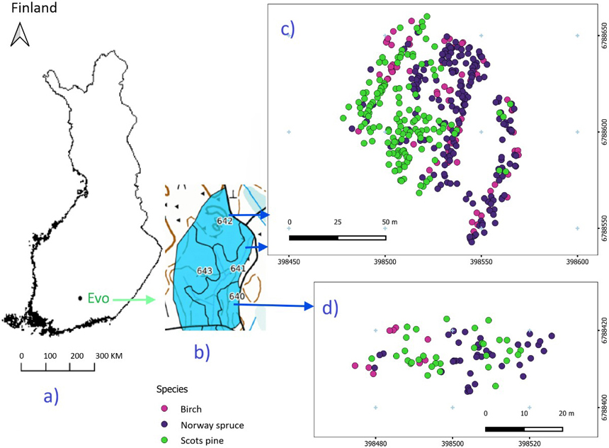
Fig. 1. Study area (a) and forest stands (b), with harvested tree species from the northern (c) and southern (d) parts.
2.2 Laser scanning systems and data collection
Three laser scanning systems were used in this study: Zenmuse L2 for DLS, Faro Orbis for BpMLS, and Ouster OS0-128 for HarvMLS. The Zenmuse L2 was operated in penta-record mode (up to five returns per pulse) mounted on a drone (DJI Matrice 350 RTK; Fig. 2). Data acquisition was performed at a flight height of 50 m above ground level (AGL), with a flight speed of 7.9 m s–1. Adjacent flight lines were designed with a 74% side overlap to provide adequate point cloud coverage. The point cloud rate was 240 000 points s–1 for single returns and 1 200 000 points s–1 for multiple returns. The inertial navigation system, with a calibrated inertial measurement unit (IMU) enabled, had an update frequency of 200 Hz. Post-processing was conducted using DJI Terra, and point clouds data were extracted in LAS format. The Zenmuse L2 provides 2 cm ranging accuracy at 150 m flight height. It operates at a 905 nm laser wavelength with 0.2 mrad horizontal and 0.6 mrad vertical beam divergence (Optron 2025).
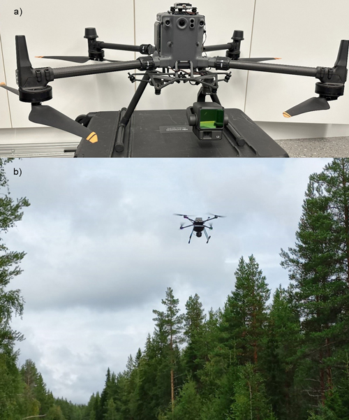
Fig. 2. Drone-based laser scanning (DLS) setup and forest scanning: Zenmuse L2 laser scanner with DJI Matrice 350 RTK drone (a), and forest scanning with DLS (b).
The Faro Orbis (Fig. 3) features a 360° × 290° field of view, mobile and stationary flash scanning systems, and a scanning range of 120 m. The BpMLS operates in the single return per pulse mode with a point cloud acquisition rate of 640 000 points s–1. The system incorporated GeoSLAM’s simultaneous localization and mapping (SLAM) algorithm, enabling real-time mapping and automatic localization during data acquisition. The FARO Connect software was used to export point clouds in a LAS format. The Faro Orbis offers a precision of 5 mm in mobile scanning and 2 mm in stationary flash scanning. It employs a 905 nm laser with a 0.7 mrad horizontal and 1.7 mrad vertical beam divergence (Faro 2025).
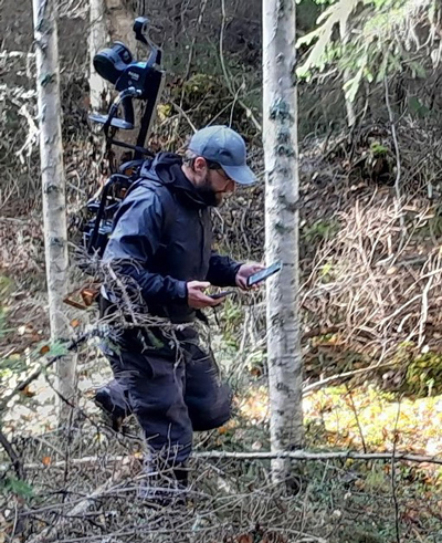
Fig. 3. Forest scanning with backpack Faro Orbis mobile laser scanner.
Two Ouster OS0-128 laser scanners were set up on the side of the crane at a 45° angle relative to the crane (Fig. 4). The scanner has a scanning capability of up to 100 m with a point cloud rate of 5.2 million points s–1. The system records the two strongest returns per pulse and provides a 360° horizontal and 90° vertical field of view. It provides an accuracy of ±0.5–5 cm, operating at an 865 nm wavelength with a 6 mrad beam divergence (General Laser 2025).
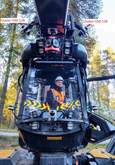
Fig. 4. Two Ouster OS0-128 LiDARs set up on Ponsse Scorpion harvester.
During the thinning operation, HarvMLS continuously scanned the forest, acquiring point cloud data in a strip-wise manner. For each strip, 3–5 consecutive point cloud datasets (LAZ files) were generated during 13–18 minutes of scanning. The first LAZ file typically represented pre-thinning conditions, whereas the last represented post-thinning conditions. Intermediate files contained a mixture of standing and harvested trees.
2.3 Point cloud processing
2.3.1 Point cloud preprocessing and co-registration
Each point cloud dataset was preprocessed using LAStools (Isenburg, 2019) for noise filtering, ground classification, and height normalisation (Fig. 5). Noise removal was implemented with the lasnoise function in LAStools with a grid spacing of 2 m horizontally and 1 m vertically. Points with <10 neighboring returns were identified as isolated and classified as potential noise for removal. Ground classification was conducted using the lasground_new function with parameters optimized for fine-scale accuracy. A 2 m grid was used, with thresholds of 1.5 m for bulges, 1 m for spikes, 0.3 m for downward spike, and an offset of 0.05 m. The ultrafine resolution mode was selected to achieve precise differentiation between ground and non-ground points, enhancing the reliability of the digital terrain representation. Next, the lasheight function was used to normalise point heights relative to the classified ground surface. The overall preprocessing approach followed the procedures described by Kafle et al. (2025) to ensure methodological consistency and comparability with previous research.
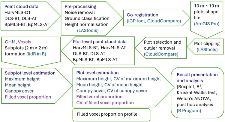
Fig. 5. Workflow of this study. The process begins with the acquisition of point cloud data and proceeds through pre-processing, processing, and analysis stages. Point cloud data were collected using harvester-mounted mobile laser scanning (HarvMLS), backpack mobile laser scanning (BpMLS), and drone-based laser scanning (DLS). HarvMLS data were obtained during thinning (DT), while DLS and BpMLS data were collected both before thinning (BT) and after thinning (AT). The study adopted open-source tools and packages, including LAStools, Cloudcompare, ArcGIS Pro, lidR, and R Studio.
Height-normalised BpMLS and HarvMLS point clouds were co-registered with the DLS point clouds using the iterative closest point (ICP) algorithm in CloudCompare (64-bit edition, version 2.13.2) (Mueller et al. 2026). The algorithm was applied with a 50% overlap to optimize alignment accuracy and reduce spatial discrepancies between the laser scanning systems (CloudCompare 2025). Accuracy was 0.07–0.16 m for BpMLS and 0.06–0.21 m for HarvMLS. The normalised DLS point cloud from the thinned area was spatially segmented and clipped in CloudCompare (Supplementary file S1: Fig. S1).
2.3.2 Plot-level point cloud processing
The clipped DLS dataset was subdivided into 10 m × 10 m grid cells, defined as study plots, and exported as a shapefile using ArcGIS Pro (Esri, 2025). This plot size was selected based on the limited thinned area (ca. 0.7 ha) and a curved north–south road along one side that restricted the use of larger plots. Individual sample plots were extracted from the processed LAS datasets using the lasclip function in LAStools.
To ensure sufficient point cloud density and minimize potential occlusion effects, plot selection was restricted to areas within a 20 m radius of the harvester’s operational path. This criterion yielded a total of 62 sample plots (10 m × 10 m), capturing both pre- and post-thinning forest structures (Suppl. file S1: Figs. S2 and S3). The spatial correspondence of the HarvMLS plots with the BpMLS and DLS plots was visually evaluated, and no discrepancies were observed for the pre-thinning forest structure. However, for the post-thinning structure, discrepancies were identified in three plots, where trees that had been harvested were still represented as standing trees in the HarvMLS data compared with the BpMLS and DLS datasets. To address this issue, the affected HarvMLS plots were segmented using GPS time information in CloudCompare, retaining only the points recorded during the last four minutes of scanning. This procedure successfully removed the erroneously retained standing trees and improved the representation of the post-thinning forest structure. For each plot, the before-thinning (BT) and after-thinning (AT) point clouds were processed independently. Based on a visual assessment, the removal of residual noise in the HarvMLS was performed in CloudCompare using the statistical outlier removal (SOR) tool. For the pre-thinning HarvMLS datasets, we applied neighborhood size (k) of 10 and a standard deviation (SD) threshold (σ) of 3 due to higher noise levels. SOR settings of 10:6 (k:σ) were selectively applied to the post-thinning HarvMLS and BpMLS point clouds because of lower noise levels. The DLS datasets showed negligible noise and did not require additional filtering.
The final selected plots had high point cloud densities (points m–2): on average, 37 235 for HarvMLS pre-thinning, 15 870 for HarvMLS post-thinning, 53 898 for BpMLS pre-thinning, 55 028 for BpMLS post-thinning, 5174 for DLS pre-thinning, and 2785 for DLS post-thinning. The higher pre-thinning point cloud densities for HarvMLS and DLS were due to denser vegetation before harvesting. However, BpMLS’s pre-thinning point cloud density was slightly lower than post-thinning, likely due to high CC significantly limiting the field of view of BpMLS that operated at 2 m above ground during pre-thinning conditions. The HarvMLS and BpMLS systems operated in single-return mode, whereas the DLS system provided up to five return modes. For the DLS dataset, all returns were used to improve the characterisation of canopy structure and height heterogeneity, as suggested by Mura et al. (2015).
2.4 Quantification of forest structure
Forest structure was quantified using eight structural attributes. The height-related attributes, maximum height, maximum height CV, mean height, and mean height CV, represent vertical structure and its variability. CC and its CV value capture horizontal structure and its variation. FVP and its CV value reflect vegetation abundance or the volumetric composition of the forest. In addition, a vertical profile of FVP was derived at the plot-level. Structural attributes were derived using grid-level approaches, including canopy height model (CHM)-based and voxel-based methods (Cimdins et al. 2025b), with the lidR package (Roussel et al. 2024) in R version 4.5.1 (R Core Team 2025).
2.4.1 CHM-based approach
Canopy height and cover attributes were derived using a CHM-based approach. A 20 cm resolution CHM (Gyawali et al. 2022) was generated using the point-to-raster (p2r) algorithm to capture fine-scale canopy structure. To obtain plot-level attribute estimates and CV values, each 10 m × 10 m CHM raster was subdivided into 2 m × 2 m subplots (4 m2 each; 25 subplots per plot), following the methodology presented by Cimdins et al. (2025b) (Fig. 6a, b). The subplot size was chosen to capture intra-plot variability while maintaining sufficient replication for reliable CV estimation.
Subplot-level maximum height was estimated as the 99.9th percentile of pixel-level CHM heights to minimise the influence of outliers (Zhang et al. 2024). Mean subplot height was obtained by averaging the pixel-level mean CHM heights. Plot-level maximum height was estimated as the highest subplot maximum height within each plot. Mean plot height was computed as the average of its subplot mean heights. CVs for maximum and mean height at the plot-level were calculated by dividing the SD across subplots by the respective plot-level mean values.
CC at the subplot-level was estimated by dividing the number of canopy pixels by the total number of pixels exceeding 3 m in height. A canopy pixel was defined as a pixel containing at least one vegetation point cloud. Previous studies have applied different height thresholds depending on vegetation density: for example, 2 m for sparse understory, 5 m for dense understory including shrubs (Dai et al. 2022), and 3 m for boreal forests (Cimdins et al. 2025b). We selected a 3 m threshold to maintain consistency with previous studies conducted under similar conditions. Plot-level CC was calculated as the mean CC across subplots. The CV of CC was calculated as the SD across subplots divided by the plot-level CC.
2.4.2 Voxel-based approach
The voxel size was set to 20 cm, consistent with the 20 cm CHM pixel size and previous studies (Juchheim et al. 2017; Cimdins et al. 2025b). For each subplot, FVP was defined as the proportion of filled voxels (voxel containing at least one point) relative to the theoretical number of voxels determined by the subplot’s maximum height. Plot-level FVP and its CV values were subsequently derived from the subplot values, following the same framework as CHM-derived structural attributes such as mean height and CC. This subplot-based framework also served to minimise potential discrepancies between theoretical and observed voxel occupancy (Fig. 6c).
At the plot-level, FVP was further evaluated across discrete vertical strata up to 20 m (FVP Profile), as only five plots exceeded this height. The FVP profile is defined as FVP computed across height intervals to characterize the vertical distribution of vegetation density. It quantifies variation in vegetation density across canopy and sub-canopy layers and identifies denser and sparser strata. The vertical stratification included 5 m canopy layers with non-overlapping intervals: up to 4.99 m, 5–9.99 m, 10–14.99 m, and 15–20 m (Fig. 6d). Subplot division was not applied in this vertical analysis to maintain comparability across height strata.
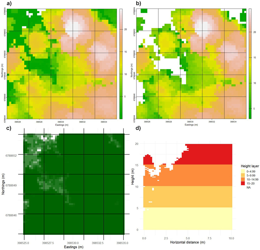
Fig. 6. Division of a sample plot (10 m × 10 m) into subplots and vertical strata to quantify forest structure. The plot was subdivided into 2 m × 2 m subplots, and canopy height models (CHMs) were generated within each subplot to estimate height (a) and cover attributes (b). Top-down view showing filled voxel proportion at the subplot scale (c). Filled voxel proportion at different height levels were computed using a voxel size of 20 cm (d). Subplot-level values were further used to calculate mean values and coefficients of variation (CVs). View larger in new window/tab.
2.5 Statistical analyses
Linear relationships and consistencies among the laser scanning systems were assessed using R version 4.5.1 (R Core Team 2025). Linear relationships between HarvMLS, BpMLS, and DLS were evaluated pairwise for the estimated forest structural attributes and structural complexity (CV) using the coefficient of determination (R2) (Pennsylvania State University 2018). The DLS data were used as the reference to calculate R2 and mean difference (MD) values when comparing HarvMLS with DLS data or BpMLS with DLS data. For comparisons between HarvMLS and BpMLS, the latter was used as the reference. MD was calculated as the mean of the test system minus the mean of the reference system (HarvMLS–DLS, HarvMLS–BpMLS, and BpMLS–DLS comparisons).
To test the consistencies or differences, we proceeded with one-way analysis of variance (ANOVA) (Heiberger and Neuwirth 2009). The ANOVA assumptions of residual normality and homogeneity of variance were assessed with the Shapiro–Wilk and Levene tests, respectively (Levene 1960; Shapiro and Wilk 1965; Niedermaier et al. 2022). When the normality assumption was violated, logarithmic, square-root, and Box–Cox transformations were applied to normalize the residuals. If the transformed data still failed the normality test, the Kruskal–Wallis nonparametric test was used (Kruskal and Wallis 1952). When the normality assumption was satisfied but the homogeneity of variances assumption was violated, Welch’s ANOVA was applied (Delacre et al. 2019). Post hoc pairwise analyses were performed using Dunn’s test following the Kruskal–Wallis test and the Games–Howell test following Welch’s ANOVA. Statistical significance was determined at a 0.05 significance level for all tests.
3 Results
3.1 Quantification of forest structure
The maximum canopy height recorded in the study area was 25.79 m. The average maximum canopy height was 17.15 m before thinning and 16.66 m after thinning, indicating minimal change in the upper canopy. This showed that the tallest trees were largely retained, with removals occurring primarily within the sub-canopy. Mean canopy height, derived from the three laser scanning systems, ranged from 9.1 to 9.8 m before thinning. After thinning, it decreased to 7.33 m due to the removal of mid-height trees. CC values from the three systems collectively declined from 0.86 to 0.68, reflecting an increase in canopy openness after thinning. Pre-thinning FVP varied among scanning systems, from 0.38 to 0.49, and declined after thinning to 0.32–0.40. An increase in CV values for height, CC, and FVP was observed across all laser scanning systems after thinning (Fig. 7). The CV of mean height increased the most, exceeding 1 in some cases, indicating greater vertical heterogeneity and variability in canopy height distribution after thinning. Overall, all laser scanning systems detected post-thinning changes in the vertical, horizontal and volumetric components of the forest structure.
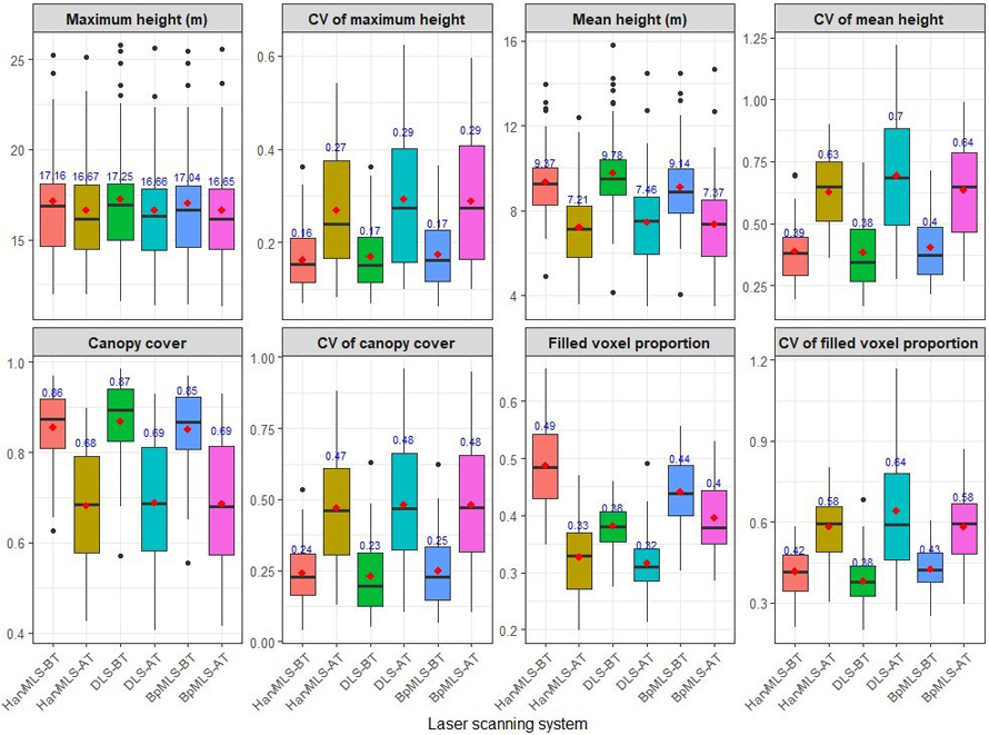
Fig. 7. Forest structural attributes quantified before and after thinning using three laser scanning systems. The assessed attributes included maximum height, mean height, canopy cover, and filled voxel proportion, with the coefficient of variation (CV) calculated for each attribute. Data were obtained from a harvester-mounted mobile laser scanner (HarvMLS), a drone-based laser scanner (DLS) and a backpack mobile laser scanner (BpMLS). Conditions are shown before thinning (BT) and after thinning (AT), with mean values indicated in red.
Analysis of FVP profiles showed that vegetation density was highest within the 5–9.99 m height interval (FVP-BT 0.42–0.48; FVP-AT 0.27–0.33) compared to other height classes (0–4.99 m, 10–14.99 m, and 15–20 m; Fig. 8). At lower heights (<5 m) and mid-height (5–9.99 m), ground-based laser scanning systems, HarvMLS and BpMLS, exhibited higher FVP compared to DLS. For the upper canopy level (>10 m), DLS showed more FVP compared to HarvMLS and BpMLS. These patterns highlighted system-specific differences in structural detection. HarvMLS and BpMLS better characterised lower canopy and understory vegetation, whereas DLS more effectively captured structure within the mid- to upper canopy layers.
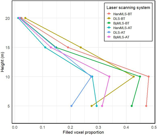
Fig. 8. Filled voxel proportion values across the different heights. Data were obtained from a harvester-mounted mobile laser scanner (HarvMLS), a backpack mobile laser scanner (BpMLS) and a drone-based laser scanner (DLS). Conditions are shown before thinning (BT) and after thinning (AT).
3.2 Linear relationships and consistencies between laser scanning systems
Canopy height attributes (maximum height, mean height, CV of maximum height, and CV of mean height) exhibited strong linear relationships between laser scanning systems (R2 0.84–0.99; Suppl. file S1: Figs. S4a, S4b, S4c, S4d). These high R2 values indicated that a large proportion of the variance in measurements from DLS or BpMLS can be explained by the measurements from HarvMLS. CC and its CV value also demonstrated very strong agreement (R2 0.94–0.99; Suppl. file S1: Figs. S4e, S4f). FVP showed a weak linear relationship across systems (R2 0.29–0.49; Suppl. file S1: Fig. S4g). The CV of FVP showed moderate to strong linear agreement between systems (R2 0.63–0.82; Suppl. file S1: Fig. S4h). Mean differences were generally higher for the structural attributes compared with the structural variability metrics. Relative to DLS, HarvMLS and BpMLS showed slight underestimation of canopy height and CC, but a slight overestimation of FVP.
The linear agreement in FVP between the laser scanning systems varied across canopy height classes (R2 0.50–0.82; Suppl. file S1: Fig. S5). In the <5 m layer, linear agreement was moderate (R2 0.50–0.68; Suppl. file S1: Fig. S5a). It improved in the 5–9.99 m (R2 0.58–0.77; Suppl. file S1: Fig. S5b) and 10–14.99 m (R2 0.61–0.75; Suppl. file S1: Fig. S5c) layers and was strongest in the 15–20 m layer (R2 0.59–0.82; Suppl. file S1: Fig. S5d). Except for the <5 m height class, HarvMLS and BpMLS showed stronger linear relationships with DLS than the HarvMLS–BpMLS comparison. Mean differences were small to moderate (MD 0–0.14). Compared with DLS, HarvMLS and BpMLS showed overestimation of FVP below 10 m, while DLS produced higher FVP estimates above 10 m.
FVP below 5 m height satisfied the normality assumption (W = 0.996, p = 0.656) but failed the homogeneity of variance test; therefore, Welch’s ANOVA was used. The remaining attributes did not satisfy the normality assumption, and data transformation attempts were unsuccessful. These attributes were analyzed using the Kruskal–Wallis test. Statistical analysis yielded comparable estimates of maximum and mean canopy height, their CVs, CC, CV of CC, CV of FVP, and FVP for the 15–20 m height class (p = 0.296–0.958). Significant differences (p = 7.8e–12) were detected between systems for FVP and FVP in <5 m, 5–9.99 m, and 10–14.99 m. A post hoc test indicated no significant difference (p = 0.103–0.565) between HarvMLS and BpMLS in the estimation of FVP and FVP profile (Table 1).
| Table 1. Results of Kruskal–Wallis test and Welch’s ANOVA for forest structural attributes derived from harvester-mounted mobile laser scanner (HarvMLS), backpack mobile laser scanner (BpMLS) and drone-based laser scanner (DLS). Chi-square value (χ2) and F value are reported for the Kruskal–Wallis test (K–W) and Welch’s ANOVA (W) test, respectively. CV denotes coefficient of variation. Significant p-values are indicated in bold. | ||||||
| Forest structural attribute | Test value | p-value | Adjusted p-value | Statistical analysis | ||
| HarvMLS vs DLS | BpMLS vs DLS | BpMLS vs HarvMLS | ||||
| Maximum height | 0.423 | 0.809 | 1.00 | 0.889 | 0.834 | K–W |
| CV maximum height | 0.592 | 0.743 | 0.939 | 1.00 | 0.670 | K–W |
| Mean height | 2.053 | 0.358 | 0.435 | 0.257 | 1.00 | K–W |
| CV mean height | 0.068 | 0.966 | 1.00 | 1.00 | 1.00 | K–W |
| Canopy cover (CC) | 0.914 | 0.633 | 0.561 | 0.679 | 1.00 | K–W |
| CV of CC | 0.210 | 0.899 | 1.00 | 0.971 | 1.00 | K–W |
| Filled voxel proportion (FVP) | 51.224 | <0.001 | <0.001 | <0.001 | 0.103 | K–W |
| CV of FVP | 2.398 | 0.301 | 0.272 | 0.267 | 1.00 | K–W |
| FVP profile | ||||||
| <5 m | 115.58 | < 0.001 | <0.001 | <0.001 | 0.483 | (W) test |
| 5–9.99 m | 9.004 | 0.011 | 0.129 | 0.004 | 0.303 | K–W |
| 10–14.99 m | 23.11 | <0.001 | <0.001 | <0.001 | 0.565 | K–W |
| 15–20 m | 1.377 | 0.502 | 1.00 | 0.431 | 0.503 | K–W |
4 Discussion
This study evaluated the performance of harvester-mounted mobile laser scanning (HarvMLS) in quantifying forest structure in a boreal forest undergoing thinning operations. Standardized metrics for forest structure remain limited, and existing indices are difficult to translate (Aalto et al. 2023; Moudrý et al. 2023). Therefore, we assessed key structural attributes representing horizontal, vertical, and volumetric forest structure and their variability. These included maximum and mean canopy height, canopy cover (CC), filled voxel proportion (FVP), and their coefficient of variation (CV). Height and cover attributes were derived using 20 cm grids, while FVP was derived using 20 cm voxels. HarvMLS produced comparable estimates of canopy height, CV of canopy height, CC, CV of CC, CV of FVP, and FVP at the upper canopy layer (15–20 m) showing moderate to strong relations (R2 0.59–0.99) with backpack mobile laser scanning (BpMLS) and drone-based laser scanning (DLS). Significant differences among the laser scanning systems were observed for total FVP and for FVP measured within the <5, 5–9.99, and 10–14.99 m height categories. Post hoc analysis, however, revealed comparable values of FVP and FVP profiles between HarvMLS and BpMLS.
Studies evaluating HarvMLS for forest structure assessment across all vegetation layers are limited, precluding direct comparisons with prior HarvMLS research. Given this limitation, we compare our findings with those of Cimdins et al. (2025b) for two primary reasons. First, both studies were conducted in Evo, Finland. The study sites were close to each other (our study: 61°21´N, 25°11´E; Cimdins et al.: 61°11´N, 25°06´E) and represented similar forest conditions. Second, both studies included airborne laser scanning data. Cimdins et al. (2025b) reported consistent estimates of the CVs of mean canopy height, CC, and FVP between helicopter-borne laser scanning (Heli-ALS: VQ-840-G, VUX-1HA, and MiniVUX-3UAV) and TLS (Leica RTC360 3D). The prediction accuracies were moderate (R2 0.395–0.583). Our study also showed consistent estimates among HarvMLS, BpMLS, and DLS for the same attributes, with significantly higher prediction accuracies (R2 0.63–0.99). Based on these two studies, forest structural variability appears to be reliably estimated using both ground-based and airborne laser scanning systems under similar forest conditions. However, further evaluation across diverse forest types and sensor configurations is needed to confirm these findings.
Previous studies have demonstrated that MLS can estimate height attributes comparable to those obtained from field measurements or ALS- or TLS-derived point cloud data. Liikonen et al. (2026) reported a very strong Pearson’s correlation coefficient (r > 0.97) between tree heights estimated using MLS (Faro Orbis) and an electronic clinometer in Heinävesi, Finland. Similarly, Holvoet et al. (2025) found a high coefficient of determination (R2 0.976) between MLS (ZEB Horizon RT) and fused MLS–DLS (DJI Zenmuse L1) data. Vandendaele et al. (2022) also reported a strong relationship (R2 0.93) between MLS (Velodyne VLP-16 Lite) and TLS (FARO Focus3D S120) for tree height estimation. These findings are consistent with the present study, showing high agreement among DLS, BpMLS, and HarvMLS in estimating height attributes. The strong agreement observed in our study is likely influenced by the relatively moderate tree heights within the study area, where the average maximum plot height was 17.1 m. Hyyppä et al. (2020) reported that MLS (GeoSLAM ZEB Horizon) increasingly underestimated tree height above 25 m under boreal forest conditions. Given these findings, evaluating the performance of HarvMLS and BpMLS in taller forests (>25 m) would be a valuable direction for future research.
The performance of MLS and DLS in tree height estimation can vary with forest structural characteristics, particularly stand composition (Mîzgaciu et al. 2025). Mîzgaciu et al. (2025) reported high prediction accuracy for MLS (GeoSLAM ZEB Horizon) in single-species stands (R2 0.93), whereas lower relationships were observed in mixed-species stands (R2 0.46–0.80). Similarly, the mean canopy height derived from a DLS (DJI Zenmuse L1) showed R2 values of 0.619 in single-species stands and 0.149 in mixed-species stands against field-measured tree heights. These results were obtained in high-canopy forests with maximum tree heights of up to 48 m (Mîzgaciu et al. 2025). Our study was conducted in mixed-species, multi-layered forest stands with relatively short canopies, with an average maximum canopy height of 17.15 m. Despite the structural complexity of these stands, DLS, BpMLS, and HarvMLS produced consistent estimates of plot-level canopy height and height variability. These results show that all three laser scanning systems reliably characterize forest vertical structure in structurally complex forests with modest canopy heights.
Previous studies have not reported the application of MLS for CC estimation. In the present study, no significant differences were observed among HarvMLS, BpMLS, and DLS in estimating CC, indicating that the ground-based mobile laser scanning systems are comparable to DLS for canopy-level attributes. These findings demonstrate the potential of BpMLS and HarvMLS for canopy structure characterization, extending BpMLS applications beyond understory structure, DBH, crown area, and tree height (Balenović et al. 2021; Vatandaşlar et al. 2023; Faitli et al. 2024; Post et al. 2025).
The ground-based systems (HarvMLS and BpMLS) yielded significantly different FVP and FVP profile estimates from DLS. This discrepancy is due to the limited ability of DLS to detect understory vegetation because of occlusion by overstory foliage, resulting in omission errors and incomplete sampling of tree stems (Hamraz et al. 2017; Muhojoki et al. 2024). However, no significant differences were found among HarvMLS, BpMLS, and DLS for FVP in the 15–20 m canopy stratum, canopy height attributes, and CC. These results indicate that BpMLS and HarvMLS provide estimates of upper-canopy structure comparable to those of DLS.
5 Conclusion
HarvMLS demonstrated reliable performance for quantifying forest structure using a grid-based approach. By continuously acquiring point cloud data during thinning, HarvMLS provided high-resolution three-dimensional characterisation of forest stand structure before and after thinning. HarvMLS showed strong agreement with DLS and BpMLS in estimating canopy height and canopy cover. furthermore, all three systems produced consistent estimates of variability for canopy height, cover, and filled voxel proportion (FVP). For volumetric forest structure, significant differences were observed between the ground-based systems (HarvMLS and BpMLS) and DLS based on FVP estimates. However, HarvMLS and BpMLS showed consistent estimates of FVP. Overall, the results demonstrate the potential of HarvMLS for detailed and reliable forest structure assessment. Future studies are suggested to evaluate the performance of HarvMLS in high-canopy forests (>23 m) and across larger areas.
Authors’ contributions
Conceptualisation and study design (BK; VK; HK; KV; KK), data collection (BK; HK; HH; HH; TF; KV), raw data processing (HK; AK; TF; NK), data processing, analysis, and results derivation (BK), writing – first draft preparation (BK), review and editing (All). All authors have approved the final version of the manuscript for publication.
Acknowledgments
We sincerely thank Mr Esa Lientola and Mr Juha Mäkelä of Häme University of Applied Sciences, Evo Campus, for facilitating test site access and supporting the field experiments. We also gratefully acknowledge the support provided by the ScanForest research infrastructure.
Funding
The study was funded through the IlmoStar project (VN/27353/2022), supported by the Ministry of Agriculture and Forestry of Finland and the European Union’s NextGenerationEU program. The Finnish Geospatial Research Institute (FGI) coordinated the project in collaboration with the University of Eastern Finland (UEF), Natural Resources Institute Finland (Luke), and Ponsse Plc. Additional support was provided by Research Council of Finland projects (357906, 359172, 359175, 359404, 359554), including the UNITE Flagship (357906 and 359172).
Declaration of openness of research materials, data, and code
The point cloud data are available from Binod Kafle upon request. The R code and quantified forest structure data are openly available at https://zenodo.org/records/23491331.
References
Aalto I, Aalto J, Hancock S, Valkonen S, Maeda EE (2023) Quantifying the impact of management on the three-dimensional structure of boreal forests. For Ecol Manag 535, article id 120885. https://doi.org/10.1016/j.foreco.2023.120885.
Angelini A, Corona P, Chianucci F, Portoghesi L (2015) Structural attributes of stand overstory and light under the canopy. Ann Silvic Res 39: 23–31. https://doi.org/10.12899/asr-993.
Atkins JW, Bohrer G, Fahey RT, Hardiman BS, Morin TH, Stovall AEL, Zimmerman N, Gough CM (2018a) Quantifying vegetation and canopy structural complexity from terrestrial LiDAR data using the FORESTR R package. Methods Ecol Evol 9: 2057–2066. https://doi.org/10.1111/2041-210X.13061.
Atkins JW, Fahey RT, Hardiman BS, Gough CM (2018b) Forest canopy structural complexity and light absorption relationships at the subcontinental scale. J Geophys Res Biogeosci 123: 1387–1405. https://doi.org/10.1002/2017JG004256.
Balenović I, Liang X, Jurjević L, Hyyppä J, Seletković A, Kukko A (2021) Hand-held personal laser scanning – current status and perspectives for forest inventory application. Croat J For Eng 42: 165–183. https://doi.org/10.5552/crojfe.2021.858.
Bienert A, Hess C, Maas HG, Von Oheimb G (2014) A Voxel-based technique to estimate the volume of trees from terrestrial laser scanner data. Int Arch Photogramm Remote Sens Spat Inf Sci XL-5: 101–106. https://isprs-archives.copernicus.org/articles/XL-5/101/2014/. Accessed 10 August 2024
Bottalico F, Chirici G, Giannini R, Mele S, Mura M, Puxedde M, McRoberts RE, Valbuena R, Travaglini D (2017) Modeling Mediterranean forest structure using airborne laser scanning data. Int J Appl Earth Obs Geoinf 57: 145–153. https://doi.org/10.1016/j.jag.2016.12.013.
Bu Y, Li W, von Gadow K, Wei J, Zhao P, Yang Y, Zhou C, Wang B, Zhao X (2025) Toward a better understanding of forest spatial patterns: a generalisation of the uniform angle index. Ecol Model 503, article id 111070. https://doi.org/10.1016/j.ecolmodel.2025.111070.
Cai S, Zhang W, Jin S, Shao J, Li L, Yu S, Yan G (2021) Improving the estimation of canopy cover from UAV-LiDAR data using a pit-free CHM-based method. Int J Digit Earth 14: 1477–1492. https://doi.org/10.1080/17538947.2021.1921862.
Chianucci F (2016) A note on estimating canopy cover from digital cover and hemispherical photography. Silva Fenn 50, article id 1518. https://doi.org/10.14214/sf.1518.
Cimdins R, Yrttimaa T, Hyyppä J, Vastaranta M, Kankare V (2024) Quantifying changes in forest structural complexity using bi-temporal airborne laser scanning. Eur J Remote Sens 57, article id 2417905. https://doi.org/10.1080/22797254.2024.2417905.
Cimdins R, Yrttimaa T, Hyyppä J, Vastaranta M, Kankare V (2025a) Capturing trends in forest structural complexity development using laser scanning techniques. Trees For People 21, article id 100954. https://doi.org/10.1016/j.tfp.2025.100954.
Cimdins R, Yrttimaa T, Vastaranta M, Kankare V (2025b) Assessing forest structural complexity: insights from alternative laser scanning approaches. Scand J For Res 41: 40–53. https://doi.org/10.1080/02827581.2025.2553745.
CloudCompare (2025) CloudCompare. Version 2.13.2. https://www.cloudcompare.org/. Accessed 10 August 2024.
Dai W, Guan Q, Cai S, Liu R, Chen R, Liu Q, Chen C, Dong Z (2022) A comparison of the performances of unmanned-aerial-vehicle (UAV) and terrestrial laser scanning for forest plot canopy cover estimation in Pinus massoniana forests. Remote Sens 14, article id 1188. https://doi.org/10.3390/rs14051188.
Delacre M, Leys C, Mora YL, Lakens D (2019) Taking parametric assumptions seriously: arguments for the use of Welch’s F-test instead of the classical F-test in one-way ANOVA. Int Rev Soc Psychol 32: 1–12. https://doi.org/10.5334/irsp.198.
Esri (2025) ArcGIS Pro. https://www.esri.com/en-us/arcgis/products/arcgis-pro/overview. Accessed 12 March 2025.
Faitli T, Hyyppä E, Hyyti H, Hakala T, Kaartinen H, Kukko A, Muhojoki J, Hyyppä J (2024) Integration of a mobile laser scanning system with a forest harvester for accurate localization and tree stem measurements. Remote Sens 16, article id 3292. https://doi.org/10.3390/rs16173292.
Falkowski MJ, Evans JS, Martinuzzi S, Gessler PE, Hudak AT (2009) Characterizing forest succession with Lidar data: an evaluation for the inland northwest, USA. Remote Sens Environ 113: 946–956. https://doi.org/10.1016/j.rse.2009.01.003.
Faro (2025) Faro OrbisTM: Mobiler laser scanner. https://media.faro.com/-/media/Project/FARO/FARO/FARO/Resources/2_TECH-SHEET/2024/Orbis-Premium/CMO12127_Techsheet_OrbisPremium_AECO_A4_ENG_Web.pdf?rev=b3f137d4ecbc40e1ac5962839fa7c9db. Accessed 12 September 2025.
Finnish Forest Centre (2026) Silvicultural methods and intermediate fellings. https://www.metsakeskus.fi/en/forest-use-and-ownership/forest-management-and-fellings/silvicultural-methods-and-intermediate-fellings. Accessed 29 January 2026.
General Laser (2025) OUSTER OS0-128 Rev 7 lidar sensor. https://general-laser.at/flyers/GL_Ouster-REV7-Sensors.pdf. Accessed 12 September 2025.
Gyawali A, Aalto M, Peuhkurinen J, Villikka M, Ranta T (2022) Comparison of individual tree height estimated from lidar and digital aerial photogrammetry in young forests. Sustainability 14, article id 3720. https://doi.org/10.3390/su14073720.
Hamraz H, Contreras MA, Zhang J (2017) Forest understory trees can be segmented accurately within sufficiently dense airborne laser scanning point clouds. Sci Rep 7, article id 6770. https://doi.org/10.1038/s41598-017-07200-0.
Hartley RJL, Jayathunga S, Massam PD, De Silva D, Estarija HJ, Davidson SJ, Wuraola A, Pearse GD (2022) Assessing the potential of backpack-mounted mobile laser scanning systems for tree phenotyping. Remote Sens 14, article id 3344. https://doi.org/10.3390/rs14143344.
Heiberger RM, Neuwirth E (2009) One-Way ANOVA. In: Heiberger RM, Neuwirth E (eds) R through excel. Springer, New York, NY, USA, pp 165–191. https://doi.org/10.1007/978-1-4419-0052-4_7.
Holvoet J, Latte N, Perin J, Bastin J-F, de Lame H, Kükenbrink D, Lejeune P (2025) Mobile laser scanning in support of national and regional forest inventories Sci Remote Sens 12, article id 100316. https://doi.org/10.1016/j.srs.2025.100316.
Hui G, Zhang G, Zhao Z, Yang A (2019) Methods of forest structure research: a review. Curr For Rep 5: 142–154. https://doi.org/10.1007/s40725-019-00090-7.
Hyyppä E, Yu X, Kaartinen H, Hakala T, Kukko A, Vastaranta M, Hyyppä J (2020) Comparison of backpack, handheld, under-canopy UAV, and above-canopy UAV laser scanning for field reference data collection in boreal forests. Remote Sens 12, article id 3327. https://doi.org/10.3390/rs12203327.
Isenburg M (2019) LAStools – efficient LiDAR processing software, version 2019, academic license. https://rapidlasso.com/lastools/. Accessed 1 December 2024.
Juchheim J, Ammer C, Schall P, Seidel D (2017) Canopy space filling rather than conventional measures of structural diversity explains productivity of beech stands. For Ecol Manag 395: 19–26. https://doi.org/10.1016/j.foreco.2017.03.036.
Kaarakka L, Cornett M, Domke G, Ontl T, Dee LE (2021) Improved forest management as a natural climate solution: a review. Ecol Solut Evid 2, article id e12090. https://doi.org/10.1002/2688-8319.12090.
Kafle B, Kankare V, Kaartinen H, Väätäinen K, Hyyti H, Faitli T, Hyyppä J, Kukko A, Kärhä K (2025) Assessing the consistency of low vegetation characteristics estimated using harvester, handheld, and drone light detection and ranging (LiDAR) systems. Silva Fenn 59, article id 25013. https://doi.org/10.14214/sf.25013.
Kärhä K (2006) Effect of undergrowth on the harvesting of first-thinning wood. For Studies 45: 101–117. https://s3web.emu.ee/emuweb/emuweb/s3fs-public/2025-03/Mets_45_11_Karha.pdf. Accessed 2 May 2025.
Kärhä K, Bergström D (2020) Assessing the guidelines for pre-harvest clearing operations of understorey in first thinnings: preliminary results from Stora Enso in Finland. Eur J For Eng 6: 14–22. https://doi.org/10.33904/ejfe.645639.
Kärhä K, Malinen J, Hyyppä J, Kaartinen H (2023) Technological opportunities in measuring biodiversity during harvesting. Finnish Forest Industries. Blog post. https://www.metsateollisuus.fi/newsroom/technological-opportunities-in-measuring-biodiversity-during-harvesting. Accessed 2 May 2025.
Kärhä K, Kaartinen H, Backas J, Honkanen H, Hyyppä J, Hyyti H, Kankare V, Kinnunen V, Kukko A, Kymäläinen H, Laitinen J, Lopatin E, Pohjala J, Uro T, Vähä-Konka V, Väätäinen K (2025) Metsäkonetiedon ja -sensoreiden Tiekartta 2035 -visio. IlmoStar-hankkeen tulevaisuusraportti. [Roadmap 2035 Vision for Forest Machine Data and Sensor Technologies. The Future Report Produced by the IlmoStar Project]. Publications of the University of Eastern Finland, Reports and Studies in Science, Forestry and Technology 10/2025. http://urn.fi/URN:ISBN:978-952-61-5717-7.
Knight CA, Anderson L, Bunting MJ, Champagne M, Clayburn RM, Crawford JN, Klimaszewski-Patterson A, Knapp EE, Lake FK, Mensing SA, Wahl D, Wanket J, Watts-Tobin A, Potts MD, Battles JJ (2022) Land management explains major trends in forest structure and composition over the last millennium in California’s Klamath Mountains. Proc Natl Acad Sci USA 119, article id e2116264119. https://doi.org/10.1073/pnas.2116264119.
Koontz MJ, North MP, Werner CM, Fick SE, Latimer AM (2020) Local forest structure variability increases resilience to wildfire in dry western U.S. coniferous forests. Ecol Lett 23, article id 31922344. https://doi.org/10.1111/ele.13447.
Korhonen L, Korhonen KT, Rautiainen M, Stenberg P (2006) Estimation of forest canopy cover: a comparison of field measurement techniques. Silva Fenn 40: 577–588. https://doi.org/10.14214/sf.315.
Korhonen L, Kärhä K, Maltamo M, Malinen J, Hyyppä J, Kaartinen H, Toivonen J, Packalen P, Koivula M (2024) Kaukokartoitus ja metsäkoneiden sensorit metsien monimuotoisuusindikaattorien seurannassa. [Remote sensing and forest machine sensors in monitoring forest biodiversity indicators]. Metsätieteen aikakauskirja, article id 23010. https://doi.org/10.14214/ma.23010.
Kruskal WH, Wallis WA (1952) Use of ranks in one-criterion variance analysis. J Am Stat Assoc 47: 583–621. https://doi.org/10.1080/01621459.1952.10483441.
LaRue EA, Hardiman BS, Elliott JM, Fei S (2019) Structural diversity as a predictor of ecosystem function. Environ Res Lett 14, article id 114011. https://doi.org/10.1088/1748-9326/ab49bb.
LaRue EA, Wagner FW, Fei S, Atkins JW, Fahey RT, Gough CM, Hardiman BS (2020) Compatibility of aerial and terrestrial LiDAR for quantifying forest structural diversity. Remote Sens 12, article id 1407. https://doi.org/10.3390/rs12091407.
LaRue EA, Knott JA, Domke GM, Chen HYH, Guo Q, Hisano M, Oswalt C, Oswalt S, Kong N, Potter KM, Fei S (2023) Structural diversity as a reliable and novel predictor for ecosystem productivity. Front Ecol Environ 21: 33–39. https://doi.org/10.1002/fee.2586.
Légaré S, Bergeron Y, Paré D (2002) Influence of forest composition on understorey cover in boreal mixed-wood forests of western Quebec. Silva Fenn 36: 353–365. https://doi.org/10.14214/sf.567.
Levene H (1960) Robust tests for equality of variances. In: Olkin I (ed) Contribution to probablity and statistics: essays in honor of Harold Hotelling. Stanford University Press, Stanford, CA, USA, pp 278–292.
Liikonen L, Yrttimaa T, Erkkilä A, Paakkari J, Pitkänen T, Kotivuori E, Vastaranta M (2026) Measuring forest inventory attributes using Faro Orbis mobile laser scanner in managed boreal forests. Forestry 99, article id cpag028. https://doi.org/10.1093/forestry/cpag028.
Maeda EE, Brede B, Calders K, Disney M, Herold M, Lines ER, Nunes MH, Raumonen P, Rautiainen M, Saarinen N, Starck I, Su Y, Terschanski J, Terryn L (2025) Expanding forest research with terrestrial LiDAR technology. Nat Commun 16, article id 8853. https://doi.org/10.1038/s41467-025-63946-6.
McElhinny C, Gibbons P, Brack C, Bauhus J (2005) Forest and woodland stand structural complexity: its definition and measurement. For Ecol Manag 218: 1–24. https://doi.org/10.1016/j.foreco.2005.08.034.
Miller JD, Knapp EE, Key CH, Skinner CN, Isbel, CJ, Creasy RM, Sherlock JW (2009) Calibration and validation of the relative differenced Normalised Burn Ratio (RdNBR) to three measures of fire severity in the Sierra Nevada and Klamath Mountains, California, USA. Remote Sens Environ 113: 645–656. https://doi.org/10.1016/j.rse.2008.11.009.
Mîzgaciu L, Tudoran GM, Ciocan AE, Stăncioiu PT, Niță MD (2025) A comparative analysis of UAV LiDAR and mobile laser scanning for tree height and DBH estimation in a structurally complex, mixed-Species natural forest. Forests 16, article id 1481. https://doi.org/10.3390/f16091481.
Moudrý V, Cord AF, Gábor L, Laurin GV, Barták V, Gdulová K, Malavasi M, Rocchini D, Stereńczak K, Prošek J, Klápště P, Wild J (2023) Vegetation structure derived from airborne laser scanning to assess species distribution and habitat suitability: the way forward. Divers Distrib 29: 39–50. https://doi.org/10.1111/ddi.13644.
Mu X, Song W, Gao Z, McVicar TR, Donohue RJ, Yan G (2018) Fractional vegetation cover estimation by using multi-angle vegetation index. Remote Sens Environ 216: 44–56. https://doi.org/10.1016/j.rse.2018.06.022.
Mueller MM, Dietenberger S, Dubois C, Kaiser S, Walz P, Lenz J, Fritz O, Marx S, Thiel C, Langer M (2026) High-resolution mapping of snow depth and snow thermal insulation using low-cost UAVs in complex Arctic Urban Terrains. Arct Sci 12: 1–23. https://doi.org/10.1139/as-2025-0062.
Muhojoki J, Hakala T, Kukko A, Kaartinen H, Hyyppä J (2024) Comparing positioning accuracy of mobile laser scanning systems under a forest canopy. Sci Remote Sens 9, article id 100121. https://doi.org/10.1016/j.srs.2024.100121.
Mura M, McRoberts RE, Chirici G, Marchetti M (2015) Estimating and mapping forest structural diversity using airborne laser scanning data. Remote Sens Environ 170: 133–142. https://doi.org/10.1016/j.rse.2015.09.016.
Niedermaier KM, Atkins JW, Grigri MS, Bond-Lamberty B, Gough CM (2022) Structural complexity and primary production resistance are coupled in a temperate forest. Front For Glob Change 5, article id 94185. https://doi.org/10.3389/ffgc.2022.941851.
North MP, Kane JT, Kane VR, Asner GP, Berigan W, Churchill DJ, Conway S, Gutiérrez RJ, Jeronimo S, Keane J, Koltunov A, Mark T, Moskal M, Munton T, Peery Z, Ramirez C, Sollmann R, White AM, Whitmore S (2017) Cover of tall trees best predicts California spotted owl habitat. For Ecol Manag 405: 166–178. https://doi.org/10.1016/j.foreco.2017.09.019.
Optron (2025) Data sheet Zenmuse L2. https://optron.com/dji/wp-content/uploads/2023/11/ds_ZENMUSE-L2.pdf. Accessed 12 September 2025.
Oshio H, Asawa T, Hoyano A, Miyasaka S (2015) Estimation of the leaf area density distribution of individual trees using high-resolution and multi-return airborne LiDAR data. Remote Sens Environ 166: 116–125. https://doi.org/10.1016/j.rse.2015.05.001.
Pennsylvania State University (2018) Lesson 2: Simple Linear Regression (SLR) model. 2.8 – R-squared cautions. Penn State Eberly College of Science, Applied Regression Analysis, STAT 462. https://online.stat.psu.edu/stat462/node/98/. Accessed 2 January 2026.
Post AJ, Forbes B, Cooper Z, Faro K, Seel C, Clark M, Disney M, Bentley LP (2025) Using handheld mobile laser scanning to quantify fine-scale surface fuels and detect changes post-disturbance in northern California forests. Ecolo Indic 172, article id 113276. https://doi.org/10.1016/j.ecolind.2025.113276.
R Core Team (2025) R: a language and environment for statistical computing. R Foundation for Statistical Computing. https://www.r-project.org/.
Rautiainen M, Stenberg P, Nilson T (2005) Estimating canopy cover in Scots pine stands. Silva Fenn 39: 137–142. https://doi.org/10.14214/sf.402.
Ross CW, Loudermilk EL, Skowronski N, Pokswinski S, Hiers JK, O’Brien J (2022) LiDAR voxel-size optimization for canopy gap estimation. Remote Sens 14, article id 1054. https://doi.org/10.3390/rs14051054.
Roussel J-R, Goodbody TRH, Tompalski P (2024) The lidR package. https://r-lidar.github.io/lidRbook/. Accessed 20 March 2025.
Sagar A, Kärhä K, Einola K, Koivusalo A (2024) Assessing the potential of onboard LiDAR-based application to detect the quality of tree stems in Cut-to-Length (CTL) harvesting operations. Forests 15, article id 818. https://doi.org/10.3390/f15050818.
Seidel D, Ehbrecht M, Puettmann, K (2016) Assessing different components of three dimensional forest structure with single-scan terrestrial laser scanning: a case study. For Ecol Manag 381: 196–208. https://doi.org/10.1016/j.foreco.2016.09.036.
Shapiro SS, Wilk MB (1965) An analysis of variance test for normality (complete samples). Biometrika 52: 591–611. https://doi.org/10.2307/2333709.
Shugart HH, Saatchi S, Hall FG (2010) Importance of structure and its measurement in quantifying function of forest ecosystems. J Geophys Res 115, article id G00E13. https://doi.org/10.1029/2009JG000993.
Stephenson NL, Das AJ, Condit R, Russo SE, Baker PJ, Beckman NG, Coomes DA, Lines ER, Morris WK, Rüger N, Álvarez E, Blundo C, Bunyavejchewin S, Chuyong G, Davies SJ, Duque Á, Ewango CN, Flores O, Franklin JF, Grau HR, Hao Z, Harmon ME, Hubbell SP, Kenfack D, Lin Y, Makana JR, Malizia A, Malizia LR, Pabst RJ, Pongpattananurak N, Su SH, Sun IF, Tan S, Thomas D, Van Mantgem PJ, Wang X, Wiser SK, Zavala MA (2014) Rate of tree carbon accumulation increases continuously with tree size. Nature 507: 90–93. https://doi.org/10.1038/nature12914.
Sumnall M, Fox TR, Wynne RH, Thomas VA (2017) Mapping the height and spatial cover of features beneath the forest canopy at small-scales using airborne scanning discrete return Lidar. ISPRS J Photogramm Remote Sens 133: 186–200. https://doi.org/10.1016/j.isprsjprs.2017.10.002.
Sun X, Xu S, Hua W, Tian J, Xu Y (2022) Feasibility study on the estimation of the living vegetation volume of individual street trees using terrestrial laser scanning. Urban Fores Urban Green 71, article id 127553. https://doi.org/10.1016/j.ufug.2022.127553.
Vandendaele B, Martin-Ducup O, Fournier RA, Pelletier G, Lejeune P (2022) Mobile laser scanning for estimating tree structural attributes in a temperate hardwood forest. Remote Sens 14, article id 4522. https://doi.org/ 10.3390/rs14184522.
Vastaranta M, Holopainen M, Yu X, Hyyppä J, Hyyppä H, Viitala R (2011) Predicting stand-thinning maturity from airborne laser scanning data. Scand J For Res 26: 187–196. https://doi.org/10.1080/02827581.2010.547870.
Vatandaşlar C, Seki M, Zeybek M (2023) Assessing the potential of mobile laser scanning for stand-level forest inventories in near-natural forests. Forestry 96: 448–464. https://doi.org/10.1093/forestry/cpad016.
Vatandaslar C, Sačkov I, Murgaš V, Pajtík J, Zeybek M (2026) Estimation of stem volume and tree structural attributes using backpack LiDAR: effects of leaf-on and leaf-off conditions. Front For Glob Change 9: 1–18. https://doi.org/10.3389/ffgc.2026.1886496.
von Gadow K, Zhang CY, Wehenkel C, Pommerening A, Corral-Rivas J, Korol M, Myklush S, Hui GY, Kiviste A, Zhao XH (2012) Forest structure and diversity. In: Pukkala T, von Gadow K (eds) Continuous cover forestry. Managing Forest Ecosystems 23: 29–83. Springer, Dordrecht. https://doi.org/10.1007/978-94-007-2202-6_2.
Wang JA, Randerson JT, Goulden ML, Knight CA, Battles JJ (2022) Losses of tree cover in California driven by increasing fire disturbance and climate stress. AGU Adv 3, article id e2021AV000654. https://doi.org/10.1029/2021AV000654.
Whelan AW, Cannon JB, Bigelow SW, Rutledge BT, Meador AJS (2023) Improving generalized models of forest structure in complex forest types using area- and voxel-based approaches from lidar. Remote Sens Environ 284, article id 113362. https://doi.org/10.1016/j.rse.2022.113362.
Zadbagher E, Marangoz AM, Becek K (2023) Characterizing and estimating forest structure using active remote sensing: an overview. Adv Remote Sens 3: 38–46. https://www.researchgate.net/publication/381489363_Characterizing_and_estimating_forest_structure_using_active_remote_sensing_An_overview. Accessed 12 September 2025.
Zhang B, Fischer FJ, Prober SM, Yeoh PB, Gosper CR, Zdunic K, Jucker T (2024) Robust retrieval of forest canopy structural attributes using multi-platform airborne LiDAR. Remote Sens Ecol Conserv 10: 725–742. https://doi.org/10.1002/rse2.398.
Total of 83 references.
Send to email

