Pekka Hyvönen  ,
Jaakko Heinonen
,
Jaakko Heinonen
Estimating storm damage with the help of low-altitude photographs and different sampling designs and estimators
Hyvönen P., Heinonen J. (2018). Estimating storm damage with the help of low-altitude photographs and different sampling designs and estimators. Silva Fennica vol. 52 no. 3 article id 7710. https://doi.org/10.14214/sf.7710
Highlights
- Digital photographs taken from low altitudes are usable for monitoring storm damage
- Simple random sampling and ratio estimators resulted in similar standard errors
- Characteristics of the storm influence the optimal flight plan and which variance estimator should be used
- The developed model for simulations can be modified and utilized with future storms.
Abstract
Climate change has been estimated to increase the risk of storm damage in forests in Finland. There is a growing need for methods to obtain information on the extent and severity of storm damage after a storm occurrence. The first objective of this study was to test whether digital photographs taken from aircrafts flying at low-altitude can be utilized in locating storm-damaged areas and estimating the need for harvesting of wind-thrown trees. The second objective was to test the performance of selected estimators. Depending on distances between flight lines, plots on lines and the used estimator, the relative standard errors of storm area estimates varied between 7.7 and 48.7%. For the area for harvesting and volume of wind-thrown trees, the relative standard errors of estimates varied between 16.8 and 167.3%. Using forest area information from Multisource National Forest Inventory data improved the accuracy of the estimates. However, performance of a simple random sampling estimator and ratio estimator were quite similar. Lindeberg’s method for variance estimation based on adjacent lines was sensitive to line directions in relation to possible trends in storm-damaged area locations. Our results showed that the tested method could be used in estimating storm-damaged area provided that the network of flight lines and photographs on lines are sufficiently dense. The developed model for simulations can be utilized also with forthcoming storms as model’s parameters can be freely adjusted to meet, e.g., the intensity and extent of the storm.
Keywords
simulation;
simple random sampling estimator;
ratio estimator;
Lindeberg;
flight line
-
Hyvönen,
Natural Resources Institute Finland (Luke), Bioeconomy and environment, Yliopistokatu 6, FI-80100 Joensuu, Finland
E-mail
pekka.hyvonen@luke.fi
- Heinonen, E-mail jaakkoheinonen@gmail.com
Received 27 April 2017 Accepted 31 May 2018 Published 5 June 2018
Views 69983
Available at https://doi.org/10.14214/sf.7710 | Download PDF

1 Introduction
In the summer of 2010, there were four extraordinarily strong thunderstorms in Finland causing broad storm damage and wind throw of trees. According to the first assessment done by practical forest workers, the amount of damaged stock was first estimated to be 1–2 million m3, but was later estimated to be 5 million m3. According to the national forest inventory (NFI) sample plots, the amount of damaged growing stock was estimated to be about 8.1 million m3 (Viiri et al. 2011). Also, the preliminary estimates of damage caused by storms by Pyry (2001) and Janika (2001) were clearly underestimated compared to the final results (Ihalainen and Ahola 2003). These great differences about damage severity between the first estimates and final results indicate that there should be statistically solid method to get reliable estimate already in the first place. Storms Asta, Veera, Lahja and Sylvi (2010), Tapani and Hannu (2011), Antti (2012), Seija, Eino and Oskari (2013), Helena (2014), Valio (2015) and Salomo and Rauli (2016) have been the latest major storms in Finland. Especially the storm Tapani caused long-lasting power outages and wind throws on an area of about 5000 hectares (Hyvönen and Korhonen, 2012).
Damaged stock can increase the risk of insect injuries and damage as the trees thrown by wind are favourable breeding ground for, e.g., bark beetle (lps typographus) and pine shoot beetle (Tomicus piniperda). Another risk is that these insect species can also attack healthy trees near the damaged areas. According to the law on prevention of forest insect and fungal damage in forests (Laki metsätuhojen torjunnasta 2013), pine timber harvested between the September 1 and May 31 should be transported from the forest by July 1 and spruce timber harvested between September 1 and June 30 by the July 15 in Southern Finland. Also wind-thrown coniferous trees must be removed from the forest, if it is economically feasible and if the amount of damaged trees is above a given limit.
It has been estimated that warming of the climate will increase storm damage in Finland (Peltola et al. 1999; Talkkari et al. 2000; Kellomäki et al. 2010). The increase of damage is related to other issues rather than just the increasing number of storms. In fact, according Gregow et al. (2008) the amount of storm winds on land areas has been at the same level in Southern Finland and even diminished in Northern Finland during 1960–2000. In addition, Laapas and Venäläinen (2017) estimated the mean linear trend for the annual and maximum wind speeds for the time period of 1959–2015 decreasing 0.09 and 0.32 m s–1 decade–1. On the other hand, in marine areas the amount of storm wind events has increased. Wind speed is estimated to increase by a few percentages between September and May in the future (Gregow et al. 2011). Climate warming is also estimated to decrease the ground frost thickness and period of its occurrence (Peltola et al. 1999; Kellomäki et al. 2010). Strong winds during early winter and spring together with unfrozen soil will most probably increase the amount of wind-thrown trees as trees’ roots don’t get support from the frozen soil. In Finland, the atmospheric depression during autumn and winter will cause stormy winds and heavy rains and snow (Gregow et al. 2008). All these phenomena together will increase storm damage, especially in forests.
There are many ways to prepare for storm damage, however all damage most likely cannot be prevented. Thus, there must be effective and rapid ways to monitor and observe storm damage and to estimate the actual extent of the destruction. This base information is valuable for planning of both harvesting of wind-thrown trees and for planning of future forest management operations, such as planting of a new tree generation.
Damage information can be obtained by extensive or sampling-based field inventory. In reality, extensive inventory means laborious work and is almost impossible as there is usually a lack of resources. The field inventory of wide areas affected by storms might also be difficult or even impossible because of the limited ability to move in the area. Roads can be blocked due to wind-thrown trees and walking in the forest is laborious and even dangerous.
Inventory of forest damage caused by storms Pyry and Janika (2003) was based on sampling, where the sampling unit was the permanent sample plot of NFI9 (Ihalainen and Ahola 2003). Altogether 1849 plots were visited in the field, covering about 3.2 million hectares of forest land.
As the field inventory of storm damage is difficult, there have been experiments to monitor storm damage by observation flights (Claesson and Paulsson 2005; King et al. 2005; Parikka 2009). In the study of Claesson and Paulsson (2005) line-wise visual assessment of sample plots was done from the aeroplane by viewing the ground at certain time intervals. Distances between lines were 10 km, distances between observing points on lines about 3 km, and the observed area on the ground on each observing point about 1.5 hectare. They reported the mean relative error of 1% for the damaged tree volume for the whole area. In the experiment by Parikka (2009), location of the observed storm damage and the estimated level of the damage were recorded using specific software and a laptop PC during the flight. In both studies, the extent of the storm damage was quickly obtained but Parikka (2009) did not report the reliability of the results. Also King et al. (2005) observed storm damage by helicopter and classified the observed damage by assigning a damage level. There were difficulties in localization of the damage and therefore the collected information could not be used for automatic image interpretation.
Storm damage can be observed also visually from aerial photographs (Pellikka and Järvenpää 2003). Reliable results require photographs taken before and after the storm. If only photographs taken after the storm are used, it might be difficult to interpret whether the damage is due to a storm or not. Bi-temporal (or multi-temporal) photographs and other remote sensing materials enable the use of automatic image interpretation of storm damage and even the estimation of damage level (Hyvönen and Anttila 2006; Vastaranta et al. 2012; Honkavaara et al. 2013; Einzmann et al. 2017). Using laser scanning data, a digital surface model (DSM) can be produced after the storm and holes in the canopy can be identified (Shedd et al. 2006) or DSM’s based on data scanned both before and after the storm can be compared (Vastaranta et al. 2012; Honkavaara et al. 2013). In the study by Honkavaara et al. (2013) storm damaged areas were identified by comparing DSM before and after a storm. The before-storm DSM was computed from the national airborne laser scanning data and the after-storm DSM was derived from high-altitude aerial photographs.
There have been also experiments to use remotely sensed data from synthetic aperture radar (SAR) sensors to detect storm damage (Fransson et al. 2002; Ulander et al. 2005; Fransson et al. 2010). Results of these studies are promising, but there seems to be complication how to detect moderate changes; like wind-thrown trees lying around.
This study had two main objectives. The first objective was to examine how digital photographs taken from the aircraft flying at low-altitude by lines can be utilized in detection of storm-damaged areas and in estimation of the need for harvesting of wind-thrown trees. The second objective was to examine the performance of different estimators and how sampling intensity affects the accuracy of different estimators.
2 Material and methods
2.1 Materials
Photographs were acquired from South-East Finland located in the municipalities of Rautjärvi, Simpele and Parikkala (Fig. 1). Storms Asta (30th of July 2010) and Vera (4th of August 2010) caused large storm damage in this region. The Asta storm moved from the south-east to the north-west and the Veera storm from the south-west to the north-east. The research area, 60 000 hectares, was close to the Russian border and therefore limited by a zone where flying is not allowed. This no-fly zone makes a bend inland in the area of Lake Simpele, and therefore there was a disconnection with the two first flight lines (Fig. 1).
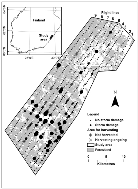
Fig. 1. Study area indicating flight lines and locations of photographs. Round symbols indicate damage severity; the size of the symbol is relative to the size of the storm area on a sample plot.
A Cessna 172N Skyhawk II aircraft was used for acquiring photographs on May 24, 2011. Altogether 673 photographs were shot with the Canon EOS 350 D digital camera that was attached to the wing strut and focused perpendicularly to the ground. The Canon ZoomBrowser EX Remote Shooting-programme running on a Panasonic Toughbook CF-19 was used to control the camera during the flight. A test flight was organized to find out the best camera parameters and flying altitude for detecting storm areas and wind-thrown trees. It was discovered that the ground resolution should be at least 12 cm in order to identify individual tree trunks. Parameters during the flight were: saving pictures only on the computer’s hard disk; picture resolution of 3456 × 2304 pixels in JPEG format; automatic focusing; 50 mm zoom level; 1/640 shutter speed and DIN 400.
With the planned flying altitude of 800 m (from the ground to the aircraft), the resolution of photographs would have been 10 cm. However, during the flight strong gusts, crosswinds and air flow unpredictably lifted and moved the aircraft. Therefore the original flight altitude was dropped to 700 m in order to have more stable flight conditions. According the saved flight data (Garmin aviation GPS) the flight altitude varied between 750 and 830 m above sea level. The terrain level varied between 80 and 140 m above sea level, so the flying altitude was on average near 700 m resulting in a ground resolution of about 9 cm on photographs. With these parameters, one photograph covered about 6.44 hectares meaning that about 7% of the study area was covered with 673 photographs.
As the test area was somewhat rectangular in shape, the flight lines were designed to follow the longest side having the direction north-east – south-west. The distances between lines were 1.5 km and distances between photographs (on the ground) varied from 478 to 590 m. The time lapse between shooting was 10 seconds when flying with a tailwind and 15 seconds with a headwind. Due to strong gusts, the airspeed varied from 65 to 110 knots (120–200 kmh–1).
2.2 Estimation of damage from sample plots on photographs
A sample plot of 90 × 90 m (0.81 ha) was placed in the centre of each photograph (Fig. 2). Three different land classes were delineated and digitized from photographs: water, forest land and other land, and the areas of these land classes in each sample plot were calculated. The proportion of storm-damage areas on the sample plot (of the whole plot area) was estimated visually. In case there were wind-thrown trees on a sample plot and no evidence that harvesting of these trees had been started, trees were digitized. In other words, a line from the bottom of the tree to the tree top was drawn. Also partly broken trees were digitized, but only the parts lying on the ground. Volumes for digitized trees were calculated using a volume model which was based on tree heights. These models were estimated from the National Forest Inventory (NFI) sample tree data. There were 542 sample plots in forested areas and 203 of those had wind-thrown trees and 28 of those had trees that needed to be harvested (Table 1). For some photographs it was not possible to assess whether the harvesting done was due to the storm or due to normal silvicultural cutting. These were further checked from the Forest Centre’s databases.
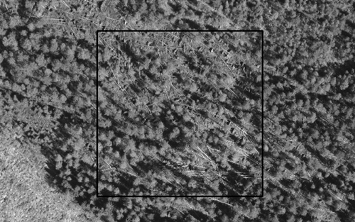
Fig. 2. Photograph taken from an altitude of 795 m. In the centre, 90 × 90 m sample plot having wind-thrown trees that need to be harvested.
| Table 1. Sample plots, amount of damaged sample plots, proportion of damage in sample plot (on average), amount of sample plots having trees and volume of trees (on a sample plot, on average) to be harvested by flight lines. | |||||
| Flight line | Sample plots | Storm damage | Not harvested | ||
| Sample plots (damaged) | Proportion of damage, % (in average) | Sample plots | m3 ha–1 (in average) | ||
| 1 | 29 | 13 | 49.6 | 2 | 9.1 |
| 2 | 70 | 28 | 36.4 | 2 | 8.1 |
| 3 | 86 | 28 | 28.3 | 3 | 19.8 |
| 4 | 87 | 25 | 25.6 | 2 | 33.0 |
| 5 | 90 | 26 | 35.6 | 4 | 27.6 |
| 6 | 84 | 18 | 45.8 | 5 | 8.6 |
| 7 | 79 | 28 | 21.8 | 6 | 2.0 |
| 8 | 78 | 19 | 22.3 | 3 | 44.1 |
| 9 | 70 | 18 | 22.2 | 1 | 1.4 |
| In total | 673 | 203 | 28 | ||
Due to the lack of proper hardware and software, photograph locations were not saved during the flight. The centre point coordinates of all photographs (and sample plots as well) were solved afterwards with the help of Google Earth, base maps and aerial photographs.
Total storm damaged area within the study area was estimated with the help of photographs. In addition, the area needing harvesting of wind-thrown trees (from here forward referred to as harvesting area) and volume of wind-thrown trees were estimated. Harvesting need was estimated based on the storm damage legislation (Laki metsän… 1991). Harvesting was regarded as necessary for a plot if there was at least one wind-thrown tree on the sample plot and additionally either 1) there was a group of at least 20 wind-thrown coniferous trees; this group might be partially outside the plot or 2) at least 10% of the coniferous trees on the plot were wind-thrown trees. Estimates for storm area and harvesting area were estimated from the sample plot data and from the sample plot data enhanced with the study area’s forest area information. These data were derived using the Multisource National Forest Inventory (MNFI) data (Tomppo et al. 2009). According to MNFI data, the forest area was 39 046 hectares comprising 64.7% of the study area.
2.3 Estimation of aerial results
The total area of storm damage, harvesting area and volume of trees for harvesting were estimated with a simple random sampling (SRS) estimator (Cochran 1977):

where A is land area, n is number of sample plots, yi is proportion of storm-damaged area (or harvesting area or volume of trees for harvesting) on sample plot i.
SRS estimator for the sampling variance was (Cochran 1977):

where ![]() is the average storm-damaged area in hectares (or harvesting area or volume of trees for harvesting) on sample plots.
is the average storm-damaged area in hectares (or harvesting area or volume of trees for harvesting) on sample plots.
The total area of storm damage was estimated also taking into account the forest area information and using a ratio estimator (Cochran 1977):
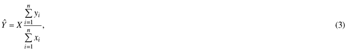
where X is the total forest area in the study area (according MNFI) and xi is the proportion of forest area on sample plot i.
The SRS estimator for the sampling variance of the ratio estimator was:
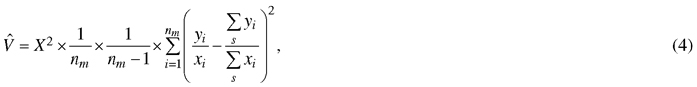
where nm is the number of sample plots with xi > 0.
SRS variance estimators may be biased because the sample method was a systematic line sampling. For that reason variances were estimated also using a Lindeberg’s equation based on differences between adjacent flight lines (Lindeberg 1924):
where p is number of flight lines and ![]() is an estimate for the whole area on the basis of flight line i. Eq. 5 estimates variance for estimator (1) if estimates
is an estimate for the whole area on the basis of flight line i. Eq. 5 estimates variance for estimator (1) if estimates ![]() are computed using Eq. 1, and variance for estimator (3), if estimates
are computed using Eq. 1, and variance for estimator (3), if estimates ![]() are computed using Eq. 3.
are computed using Eq. 3.
Standard error (SE) was computed as:
![]()
And relative standard error (RSE), was computed using the equation:
![]()
In Eq. 7 the estimator ![]() is either a SRS estimator or a ratio estimator, and standard error SE is computed using either the corresponding SRS equation or the Lindeberg equation.
is either a SRS estimator or a ratio estimator, and standard error SE is computed using either the corresponding SRS equation or the Lindeberg equation.
Due to fluctuation in flight altitude and orientation of the camera, the plot size on ground was not constant but varied around value 0.81 ha which was used in calculations. However, this variation was independent of the spatial variation of storm damage and its effect on the results is negligible.
2.4 Resampling and simulation
Estimates and the relative standard errors were calculated using the whole data. In addition, resampling and simulation was used to examine the effects of sampling design on the statistical properties of damage estimates and on relative error estimates. In resampling, no statistical model for data is needed and it was applied to all response variables. However, in resampling there were for each design only two or a few different samples and therefore the relative errors were assessed using only analytical formulas. The usefulness of resampling for examining the effect of distance between lines was not so obvious, because data included only nine lines. Resampling also did not allow testing the effect of line orientation.
A larger set of designs was examined applying simulation for damaged area estimation. Simulation provided also the comparison of the analytical estimates of relative errors to the relative errors observed in simulation.
Simulation allowed testing a larger set of alternative designs. In simulation several wall to wall datasets were generated using a statistical model for the distribution of damage on the research area. The mean values, variances and spatial correlations of the random terms of the model were estimated from the measurements of the area. All tested sampling designs were applied repeatedly to all generated datasets. Each generated dataset represent one realization of the random damage distribution on the area. The mean value of the results obtained from different realizations estimates the expected values of the results and they are applicable to the actual damages on the area. The mean values are also comparable to the results obtained by resampling.
2.4.1 Resampling
In resampling, subsamples were selected from the photograph data according to different sampling designs. A design included either all the sample plots on a flight line or only every 2nd, 3rd, 4th, 5th or 6th sample plot corresponding to distances between sample plots 0.5, 1, 1.5, 2, 2.5 and 3 km, respectively. In different designs distances between lines were 1.5 km, 3 km, 4.5 km or 6 km. The corresponding line combinations in a sample were:
all lines (gap between flight lines 1.5 km)
lines 1–3–5–7–9 and 2–4–6–8 (gap between flight lines 3 km)
lines 1–4–7, 2–5–8 and 3–6–9 (gap between flight lines 4.5 km)
lines 1–5–9, 2–6, 3–7 and 4–8 (gap between flight lines 6 km)
Altogether 24 ( = 6 × 4) different designs were examined. The number of samples corresponding to a design varied. E.g. only one sample corresponds to the design which includes all the lines and all the sample plots. Three different samples correspond to the design of every 3rd sample plot on each flight line, as the starting point on a line may be the 1st, the 2nd or the 3rd plot of the 1st line. Storm area estimates and variance estimates for a design d were the mean values:


where m is the number of samples corresponding to the design d and storm-damaged area estimate ![]() and variance estimate
and variance estimate ![]() were computed from sample i of design d. Relative standard errors corresponding to a design d were computed using Eq. 6 and 7.
were computed from sample i of design d. Relative standard errors corresponding to a design d were computed using Eq. 6 and 7.
2.4.2 Simulation
The study area was covered with grid-network using squares of 90 × 90 metres cell size, which was the size of the sample plots on the photographs. For every square, proportion of forest area was determined with the help of a MNFI land use map. The proportion of storm-damaged area was generated for every forest square (forest area > 0) using a spatial random field model which was based on the sample plots. The spatial correlation structure of storm area was assessed by fitting variogram for the proportional damage areas on the plots. The variance of the random variation around the expected value of proportional damage area was modelled as a function of it’s expected value. The model was developed using one out kriging residuals of forest sample plots. The expected values of forest squares were estimated using local kriging. The proportional damage area on forest squares were generated by adding uncorrelated normal distributed random terms to the expected values. The variances of the random terms were set according to the variance model. The storm area of a forest square was computed by multiplying the generated proportional damage area with the forest area.
Given a generated data, 500 samples were drawn for each design. The storm area estimates and the variance estimates for a design, given a generated data, were computed in the same way as in the case of resampling as the mean values of the estimates computed from different samples. An additional estimate of the sampling variance was computed as the variance of the 500 replicates of the storm area estimate.
Data was generated 50 times. Each new dataset was obtained by generating a new set of random terms. Sampling was repeated for all generated data sets according to all designs. Storm area estimates for the true storm-damaged area of the study area and their variance estimates, given a design d, were the mean values:


where p = 50 and storm area estimates ![]() and variance estimates
and variance estimates ![]() were estimates given generated data J. Relative standard errors corresponding to a design were computed using Eq. 6 and 7.
were estimates given generated data J. Relative standard errors corresponding to a design were computed using Eq. 6 and 7.
A 95% range of the relative standard errors, given a simulated data and design d, was defined as the 2.5 and 97.5 percentage points of the distribution of 500 values. Corresponding percentage points for the true storm-damaged area were computed as the mean values of the 50 replicates, each replicate representing different generated data.
Only the photo sample plot values are known in the study area and therefore the mean values of a statistic over different simulated data sets estimate the corresponding statistic given the true but unknown spatial distribution of the storm-damaged area.
2.4.3 Data generation in detail.
An isotropic Matérn variogram (Matérn 1960; Minasny and McBratney 2005; Marchant and Lark 2007) was fitted for z = y/x, the ratio of storm area and forest area on photo data plots. Variance of z depends on the level of z and the variance was modelled as follows. Local live-one-out kriging estimates ![]() and residuals resi = z –
and residuals resi = z – ![]() were computed for the forest sample plots. The live-one-out estimate
were computed for the forest sample plots. The live-one-out estimate ![]() for a plot used all forest sample plots within the range of 3 km of the plot except the plot itself.
for a plot used all forest sample plots within the range of 3 km of the plot except the plot itself.
The model for the conditional standard deviation of z, given ![]() , was:
, was:
![]()
where c is a coefficient and v0 is the lower limit for the variance. The lower limit was needed because there was random variation even if the kriging estimate was ![]() = 0. The values of c and v0 were computed using Eq. 13 and 14:
= 0. The values of c and v0 were computed using Eq. 13 and 14:
![]()

Sum in Eq. 13 is over all the plots and n0 in Eq. 14 is the number of plots with ![]() ≤ 0.01.
≤ 0.01.
In simulations, local kriging estimates![]() were computed for all the forest squares in the study area using the forest sample plots within the range of 3 km of the square. The estimate of standard deviation sz was computed for all the forest squares replacing
were computed for all the forest squares in the study area using the forest sample plots within the range of 3 km of the square. The estimate of standard deviation sz was computed for all the forest squares replacing ![]() with
with ![]() in Eq. 12.
in Eq. 12.
The leave-one-out residuals were uncorrelated, and the simulated values were computed as:
![]()
where r stands for uncorrelated N(0,1) variates. A simulated proportion of storm area on a plot is y = z × x.
Normal distribution results in both negative and values larger than one, but we were interested only in the two first moments of the sampling distributions and therefore normal distribution was applicable. However, robustness of the results was examined in two different ways.
Photo data does not provide information about the spatial correlation for distances smaller than 0.5 km. To check the effect of short distance correlations on the results, simulated values were generated also using the model:
![]()
where rcor are correlated N(0,1) variates with exponential covariance function cov(dist) = exp(k × dist), where dist is distance between two squares. Values k = –0.25 and k = –0.5 were applied.
The sensitivity of the results to the higher moments of the distribution of z was examined by sampling z values also from uncorrelated beta-distributions with expected values![]() and standard deviations sz. However, if the expected value of a beta distribution is small (
and standard deviations sz. However, if the expected value of a beta distribution is small (![]() < 0.02), standard deviation of the beta distribution is necessarily smaller than sz. Therefore z was taken from Bernoulli(0.02) distribution whenever
< 0.02), standard deviation of the beta distribution is necessarily smaller than sz. Therefore z was taken from Bernoulli(0.02) distribution whenever![]() < 0.02.
< 0.02.
Visual interpretation of photographs and digitising of wind-thrown trees and land classes were done in ArcGIS. All other analysis and calculations were done using R software (v. 3.1.1, R Core Team 2014). Kriging variograms were fitted using gstat-function fit.variogram, kriging estimates were computed using krige, residual variograms were fitted using the RandomFields-function RFit and scaled residuals were simulated using the RandomFields-function RFsimulate.
3 Results
3.1 Resampling
The SRS estimate for storm-damaged area was 5634 ha. The estimated volume of wind-thrown trees for harvesting was 39 246 m3 and estimated harvesting area was 1000 ha. Ratio estimates were about 5 percents lower for all these estimates, 5345 ha, 37 233 m3 and 949 ha, respectively. As distance between sample plots was increased (and the number of sample plots on flight lines was decreased), the storm-damaged area SRS estimates varied between 5438 and 5662 ha, and the ratio estimates between 5123 and 5426 ha.
The relative standard error of the SRS estimate (SRS-SRS) of the storm-damaged area was 8.7% and the relative standard error of the ratio estimate (Ratio-SRS) was 7.7% (Fig. 3). Corresponding relative standard errors based on Lindeberg’s variance equations, SRS-Lindeberg and Ratio-Lindeberg, were very similar. Furthermore, the relative standard errors for the harvesting area were 23.9% (SRS-SRS), 20.9% (Ratio-SRS), 14.5% (SRS-Lindeberg) and 16.4% (Ratio-Lindeberg) (Fig. 4), and that of volume of wind-thrown trees for harvesting 32.7% (SRS-SRS), 27.7% (Ratio-SRS), 31.3% (SRS-Lindeberg) and 26.7% (Ratio-Lindeberg), respectively (Fig. 5).
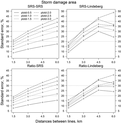
Fig. 3. Relative standard errors of storm-damaged area estimates of resampling with different estimation methods and parameters. “SRS-SRS” means simple random sampling estimator, “SRS-Lindeberg” simple random sampling estimator using Lindeberg’s adjacent line method. “Ratio-SRS” simple random sampling ratio estimator and “Ratio-Lindeberg” simple random sampling ratio estimator using Lindeberg’s adjacent line method. “plotd-0.5” means 0.5 kilometre distance between photographs on flight line, “plotd-1.0” one kilometre distance, etc.
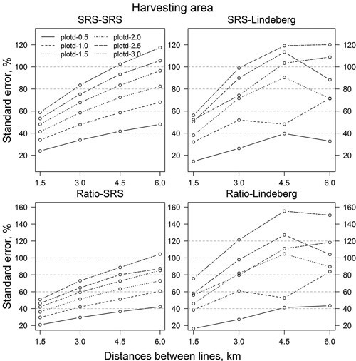
Fig. 4. Standard errors (%) of estimated harvesting area in resampling with different estimation methods and parameters. Abbreviations are as in Fig. 3.
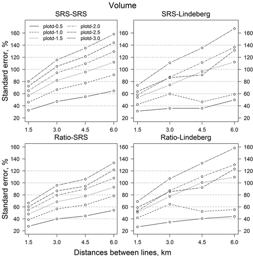
Fig. 5. Standard errors (%) of volume of wind-thrown trees for harvesting estimates with different resampling methods and parameters. Abbreviations are as in Fig. 3.
Increasing distances between sample plots or/and flight lines (that is decreasing the number of sample plots and/or flight lines) in resampling increased standard errors (Figs. 3–5). In all, standard errors of the ratio estimates were smaller than the standard errors of the comparable SRS estimates. On average, the relative standard errors were 2.6 percentage units smaller for storm area, 8.5 units for harvesting area and 15.4 units for the volume of wind-thrown trees for harvesting. RSE values based on Lindeberg’s equation were mainly bigger than the corresponding RSE values based on SRS variance estimators. For storm area the Lindeberg’s method resulted in, on average, 4.3 (SRS-Lindeberg compared to SRS-SRS) and 2.6 (Ratio-Lindeberg compared to Ratio-SRS) higher percentage unit RSE values. The differences in harvesting area were 2.8 and 22.9 percentage units, respectively. On the other hand, SRS-Lindeberg RSE values were 8.6 percentage units smaller on average than SRS-SRS RSE values for volume of wind-thrown trees for harvesting. For corresponding ratio estimates Ratio-Lindeberg values were 4.9 percentage units bigger than Ratio-SRS values.
3.2 Simulations
In the simulated data the storm area varied between 4932 and 5004 ha. The lowest relative standard errors with the densest data set, that is a line distance of 1 km and sample plot distance of 0.5 km, were 7.1% (SRS-SRS), 6.9% (Ratio-SRS), 10.8% (SRS-Lindeberg) and 8.1% (Ratio-Lindeberg) (Fiq. 6). The trend was clear and near linear; increasing line or plot distances increased the RSE values. The SRS-SRS and Ratio-SRS values were quite similar. The Ratio-SRS values were 0.3–1.3 percentage units lower than the corresponding SRS-SRS values. On the other hand, SRS-Lindeberg values were clearly higher than SRS-SRS values. On average, SRS-Lindeberg values were 5.6 percentage units higher than SRS-SRS values. Increasing the line distance had a smaller effect than increasing the plot distance on SRS-SRS and Ratio-SRS values (Fig. 6). On average, increasing the plot distance by 0.5 km increased the relative standard errors 3.5 percentage units (SRS-SRS) and 3.4 percentage units (Ratio-SRS). In Lindeberg’s method, the effect of increasing line or plot distances was opposite. Increasing the line distance by 0.5 km increased the relative standard errors on average 3 percentage units (SRS-Lindeberg) and 2.5 percentage units (Ratio-Lindeberg) and increasing the plot distance by 0.5 km increased the relative standard errors on average 2.3 and 1.8 percentage units, respectively.
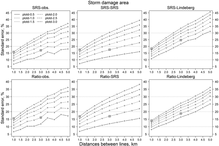
Fig. 6. Relative standard errors of storm-damaged area estimates of simulations with different estimation methods and parameters. “SRS-obs.” means variation calculated from the observed values. Squares illustrate the combination of line and plot distance of 1 km by 3 km and 3 km by 1 km, respectively. Other abbreviations are as in Fig. 3.
The same result can be observed in Fig. 7. Decreasing the number of sample plots, either by decreasing the number of lines or the number of plots on a line, increased the RSE values. Relative standard errors of SRS-SRS and Ratio-SRS were close to each other. On the other hand, the variability of the RSE values based on Lindeberg’s equation were more sensitive to the number of lines than the RSE values based on the simple random sampling assumption (SRS-SRS and Ratio-SRS). The orientations of the lines (original direction or perpendicular to it) had little effect on the confidence intervals of SRS-SRS and Ratio-SRS, whereas the variation of RSE values based on Lindeberg’s method decreased clearly when the orientation of lines was changed to perpendicular to the original orientation (Figs. 8 and 9). For example, with 1 km plot and line distances, the confidence interval of relative standard error was about 6–22% (original line directions) and 7–13% (perpendicular lines). With line distances of 5 km, the values were 5–70% and 15–45%, respectively (Figs. 9 and 10).
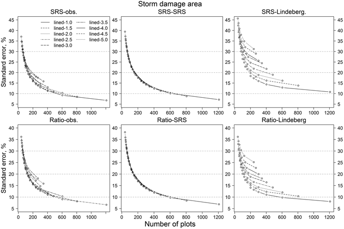
Fig. 7. The effect of number of sample plots on relative standard errors of storm-damaged area estimates in simulations. “lined-1.0” means 1 kilometre distance between lines, “lined-1.5” 1.5 kilometre distance, etc. Abbreviations are as in Fig. 6.
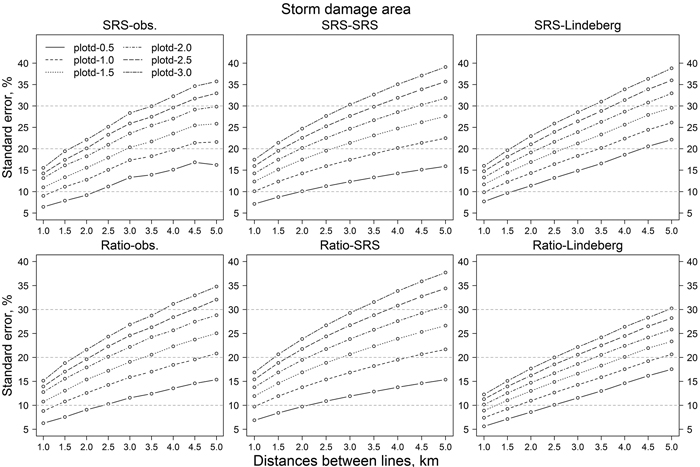
Fig. 8. Relative standard errors of storm-damaged area estimates of simulations with different estimation methods and parameters with dataset from lines turned 90-degrees compared to original lines direction. Abbreviations are as in Fig. 6.
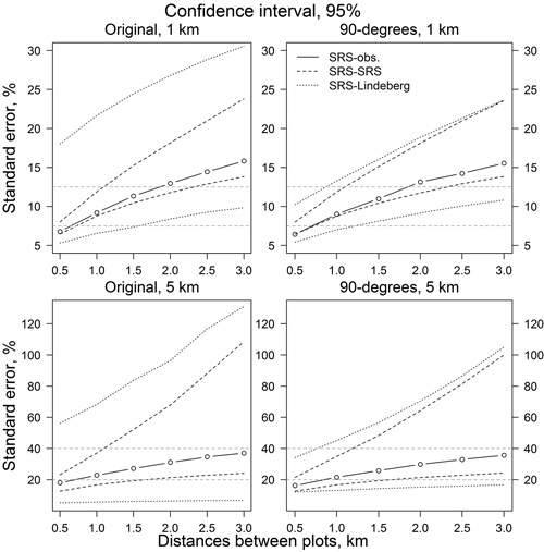
Fig. 9. Confidence intervals for relative standard error of SRS-SRS and SRS-Lindeberg’s estimates. Original line direction for 1 and 5 km line distances (left) and perpendicular to the original line direction (right). Legend abbreviations are as in Fig. 6.
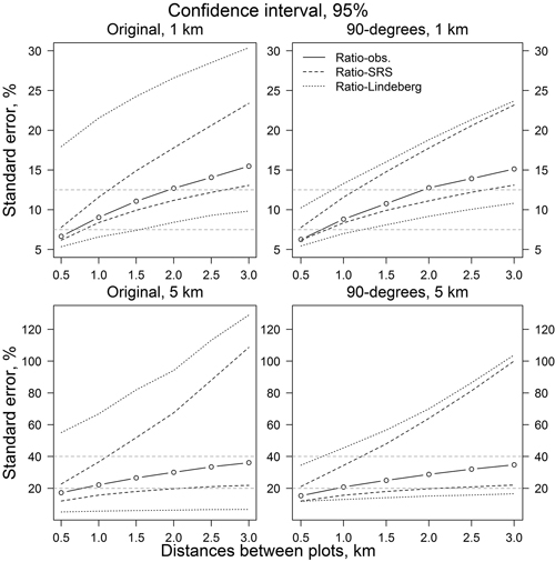
Fig. 10. Confidence intervals for relative standard error of Ratio and Lindeberg’s estimates. Original line direction for 1 and 5 km line distances (left) and perpendicular to the original line direction (right). Legend abbreviations are as in Fig. 6.
4 Discussion
Empirical data of this study was acquired by flying with light aircraft and taking digital photographs with a camera attached to the wing strut and focused perpendicularly to the ground. The flight area covered about 60 000 hectares having nine flight lines spaced at 1.5 km distances. The applied configuration worked well and was discovered to be suitable for monitoring of small areas. On the other hand, due to fluctuation in flight altitude and possible differences on camera orientation caused by strong gusts, the actual sample plot size varied around 0.81 ha. This variation was independent on the spatial variation of the storm damage and we can assume that the mean value of the plot size is close to the value of 0.81 ha and therefore it has only negligible effect on the expected values of the damage estimates. Sampling variance increases if variation of plot size increases, which wasn’t included in our variance formulas. However, the effect on proportional standard error was negligible and according to our simulations it was less than one percent unit in all sample sizes.
After the flight, the processing of photographs took time and was somewhat laborious. The most time-consuming was locating photographs and determination of coordinates for sample plots as coordinates were not attached to photograph meta-information during the flight. Also digitising of wind-thrown trees took time but was easy to do. Yet, for some trees it was difficult to determine the tree top or the actual starting point of the stem because several trees had fallen in groups. In most cases the starting point of the stem (stump/roots) could be clearly identified but not the tree top. Most likely this led to underestimation of lengths of wind-thrown trees. Thus, estimated volume of wind-thrown trees to be harvested, 37 230 m3, was probably underestimated.
The ratio estimator estimated the storm area to be 5345 ha, about 13.7% of forest area. The Ratio-SRS estimator gave, on average, standard errors that were 0.7 percentage units lower than the SRS-SRS estimator in simulations. Furthermore, Lindeberg’s ratio gave, on average, standard errors that were 6.3 percentage units lower than Lindeberg’s SRS. This means that information about forest area from the Multisource National Forest Inventory (MNFI) data improves the accuracy of the estimates.
The Lindeberg’s SRS gave, on average, standard errors that were 5.6 percentage units higher in simulations and 4.3 percentage units higher in resampling compared to SRS-SRS. An obvious reason for these results was that storm areas were concentrated on the southern part of the study area and there seemed to be some rolling or wavy variation in storm areas perpendicular to the original flight lines (Fig. 1). Lindeberg’s method should yield larger errors than SRS if the differences between adjacent lines are clear, as was the case. This same phenomenon can be seen in Fig. 3 and partly in Figs. 4 and 5. The relative standard error in resampling increases almost linearly up to 4.5 km line distances. However, with 6 km line distance the standard error stays almost at the same level or even decreases. This is due to the data and how storm-damaged areas are situated on the lines. As the line distance is 6 km, there are only 2 lines in data at the time. It can be noted from Table 1 that with those line combinations the differences between lines in storm-damaged areas and count of unharvested sample plots are not as large as with other line combinations and with other line distances. In volume of wind-thrown trees for harvesting the differences between lines are not so large and therefore the results are more logical.
In addition to rolling or wavy variation perpendicular to original flight lines, there seemed to be a trend parallel to original flight lines. This is supported by the results of simulations with lines perpendicular to the original direction of flight lines. In case differences between adjacent lines are small, Lindeberg’s equation should give smaller errors than SRS. In this data Lindeberg’s equation gave similar or a little bit smaller errors than SRS. As different estimators might give different results depending on a storm’s characteristics, there should be some background knowledge, e.g. course of the storm, to make up the optimal flight plan.
Accuracy of the results of this study, compared to the study of Claesson and Paulsson (2005), are somewhat worse. In their study, the total damaged tree volume was 69.7 million m3 and the mean relative error of that 1% for the whole area. On the province level the damaged tree volume varied between 3.2 and 22 million m3 and the relative error of that from 2% to 7%. Accurate results are most probably due to extensive data; 37 flight lines having about 2100 observation. Also in this study, the relative error of storm damage area with simulations and used estimators was 7–11% with the largest data set, about 1200 sample plots.
In order to be a useful method in practise, the relative standard errors should be less than 15% (Yu et al. 2003). This was achieved in storm area estimates with maximum flight line distances of 5 km (having a plot distance of 0.5 km) or with maximum flight line distances of 1.0 km (having a maximum plot distance of 2.5 km) in simulations. With original data and resampling the 15% limit was achieved with all combinations of flight lines having all sample plots. Also having all flight lines with at least every 4th sample plot (equal to 2 km plot distance) gave a standard error near 15%. This means that there should be enough flight lines with reasonable distances to cover the whole area. Especially in cases where damage areas are clustered, which is a typical pattern of storm damage. In this study the maximum distance between flight lines seemed to be near 2.5 to 3 km. A precondition for this is that there are enough photographs taken on each flight line. According to this study, the distance between photographs on flight lines should be not more than 1 km. If a flight line or plot distance is increased, the other distance should be decreased. Concerning the estimation of harvesting area and volume of wind-thrown trees, the sampling should be much denser. Otherwise there is no guarantee that results are sufficiently reliable.
As illustrated in Fig. 6 with square-marks, the RSE values are almost the same in cases where plot and line distances are changed the other way round: almost the same result is achieved using, e.g., 1 km line distance with 3 km plot distance or 3 km line distance with 1 km plot distance. With Lindeberg’s’ method this was not true. However, according to, e.g. Matèrn (1960), there should be enough sample units to have reliable results by using variance estimators. In this study, as the flight lines was used as a sample unit, the amount of samples was 15 and with the lines perpendicular to the original direction 41 in maximum in simulations. 15 lines seemed to be insufficient for Lindeberg’s method, whereas results with perpendicular lines were consistent with other estimators. In fact, Ratio-Lindeberg gave the lowest RSE values (Fig. 8). No good explanation for this was found.
In practise, there are no extra costs for taking more photographs on flight lines, whereas increasing the number of flight lines increases flight time and therefore costs. On the other hand, processing a large number of photographs is time consuming if no automatic or semiautomatic method is available. One possibility to reduce the laborious parts is to have a location saved on photographs during the flight and visually estimate the storm damage and forest area on a photograph and also the volume of wind-thrown trees. This way it is possible to get a quick estimate of damage severity and decide how to proceed with forest management operations.
In large-scale storm-damaged areas one option is to use aerial photographs and NFI sample plot field data. The proportion of damaged area or trees is estimated on NFI sample plot locations based on visual interpretation of aerial photographs taken after a storm. Then the volume of wind-thrown trees is calculated based on estimated damage proportion and NFI sample plot tree data. Most likely this will give quite reliable results without field visits. Acquired aerial photographs could be used also for detailed planning of management operations. One drawback of using aerial photography is that the photographing conditions might be unsuitable for a long time after the storm occurrence.
One option to get quick a first estimate of storm damage with relatively low costs might be to drive on roads and observe damage from roadsides, e.g. inside a 50-metre zone. To be a statistically sound method, this would require a model to estimate how reliably wind-thrown trees and storm area can be quantified from the road.
Our method was based on sampling. Nowadays there are increasing possibilities to obtain datasets from different time points, which can be used for change detection and for wall-to-wall map estimation purposes. In addition, different dataset can be utilized concurrently. E.g. point clouds generated from existing airborne light detection and ranging (Lidar) data (acquired before storm) and aerial photographs (acquired after storm) can be used for change detection. With these kinds of datasets it is possible to cover large areas and get reliable results. However, there must be a method to conclude which changes are due to storm and which silvicultural operations.
5 Conclusion
Digital photographs taken by following systematic sampling rules proved to be usable to estimate the area of storm damages. However, to get reliable results the amount of photographs must be adequate, which, consequently, increases the time to process the data and therefore costs. The developed model for simulations is flexible and it can be utilized with forthcoming storms. The model parameters can be freely adjusted to meet, e.g., the intensity and extent of the storm. In addition to model parameters, different design of flight lines can be tested to find the optimal flight plan for different purposes; such as to estimate the size of damage area. Developed system gives good opportunity to do thorough sensitivity analysis.
Acknowledgments
This study was part of the project “Tools to detect storm damage areas”. The authors wish to thank the Ministry of Agriculture and Forestry for the financial support.
References
Claesson S., Paulsson J. (2005). Flyginventering av stormfälld skog – januari 2005. Raport, Skogsstyrelsen. 10 p.
Cochran W. (1977). Sampling techniques. John Wiley & Sons, New York. 428 p.
Einzmann K., Immitzer M., Böck S., Bauer O., Schmitt A., Atzberger C. (2017). Windthrow detection in european forests with very high-resolution optical data. Forests 8(1): 1–26. https://doi.org/10.3390/f8010021.
Fransson J.E.S., Walter F., Blennow K., Gustavsson A., Ulander L.M.H. (2002). Detection of storm damaged forested areas using airborne CARABAS-II VHF SAR image data. IEEE Transactions on Geoscience and Remote Sensing 40(10): 2170–2175. https://doi.org/10.1109/TGRS.2002.804913.
Fransson J.E.S., Pantze A., Eriksson L., Soja M., Santoro M. (2010). Mapping of wind-thrown forests using satellite SAR images. Geoscience and Remote Sensing Symposium (IGARSS) 2010 IEEE International. p. 1242–1245. https://doi.org/10.1109/IGARSS.2010.5654183.
Gregow H., Venäläinen A., Laine M., Niinimäki N., Seitola T., Tuomenvirta H., Jylhä K., Tuomi T., Mäkelä A. (2008). Vaaraa aiheuttavista sääilmiöistä Suomen muuttuvassa ilmastossa. Ilmatieteenlaitos raportteja 2008:3. 99 p. [In Finnish].
Gregow H., Peltola H., Laapas M., Saku S., Venäläinen A. (2011). Combined occurence of wind, snow loading and soil frost with implications for risks to forestry in Finland under the current and changing climate conditions. Silva Fennica 45(1): 35–54. https://doi.org/10.14214/sf.30.
Honkavaara E., Litkey P., Nurminen K. (2013). Automatic storm damage detection in forest using high-altitude photogrammetric imagery. Remote Sensing 5(3): 1405–1424. https://doi.org/10.3390/rs5031405.
Hyvönen P., Anttila P. (2006). Change detection in boreal forests using bi-temporal aerial photographs. Silva Fennica 40(2): 303–314. https://doi.org/10.14214/sf.345.
Hyvönen P., Korhonen K.T. (2012). Myrskytuholaskennan tulokset Lounais-Suomen, Pirkanmaan ja Häme-Uusimaan alueilla. Raportti, Metsäntutkimuslaitos. 2 p. [In Finnish].
Ihalainen A., Ahola A. (2003). Pyry- ja Janika-myrskyjen aiheuttamat puuston tuhot. Metsätieteen aikakauskirja 3/2003: 385–401. [In Finnish]. https://doi.org/10.14214/ma.6803.
Kellomäki S., Maajärvi M., Strandman H., Kilpeläinen A., Peltola H. (2010). Model computations on the climate change effects on snow cover, soil moisture and soil frost in the boreal conditions over Finland. Silva Fennica 44(2): 213–233. https://doi.org/10.14214/sf.455.
King D.J., Olthof I., Pellikka P., Seed E.D., Butson C. (2005). Modelling and mapping damage to forests from an ice storm using remote sensing and environmental data. Natural Hazards 35(3): 321–342. https://doi.org/10.1007/s11069-004-1795-4.
Laapas M., Venäläinen A. (2017). Homogenization and trend analysis of monthly mean and maximum wind speed time series in Finland, 1959–2015. International Journal of Climatology 37(14): 4803–4813. https://doi.org/10.1002/joc.5124.
Laki metsän hyönteis- ja sienituhojen torjunnasta. 8.2.1991/263. [In Finnish].
Laki metsätuhojen torjunnasta. 20.12.2013/1087. [In Finnish].
Lindeberg J.W. (1924). Über die Berechnung des Mittlerfehlers des Resultates einer Linientaxierung. Acta Forestalia Fennica 25. 22 p. https://doi.org/10.14214/aff.7080. [In German].
Marchant B.P., Lark R.M. (2007). Estimation of linear models of coregionalization by residual maximum likelihood. European Journal of Soil Science 58(6): 1506–1513. https://doi.org/10.1111/j.1365-2389.2007.00957.x.
Matérn B. (1960). Spatial variation. Meddelanden från Statens Skogsforskninginstitut 49(5). 144 p.
Minasny B., McBratney A.B. (2005). The Matérn function as a general model for soil variograms. Geoderma 128(3–4): 192–207. https://doi.org/10.1016/j.geoderma.2005.04.003.
Parikka H. (2009). Laajojen myrskytuhojen kartoitus. Raportti, Metsäntutkimuslaitos. 34 p. [In Finnish].
Pellikka P., Järvenpää E. (2003). Forest stand characteristics and snow and wind induced forest damage in boreal forests. In: Ruck B. (ed.). Procedings of the International Conference On Wind Effects on Trees, Karlsruhe, Germany, 16–18 Sept. 2003. p. 269–279.
Peltola H., Kellomäki S., Väisänen H. (1999). Model computations on the impact of climatic change on the windthrow risk of trees. Climatic Change 41(1): 17–36. https://doi.org/10.1023/A:1005399822319.
R Core Team (2014). R: a language and environment for statistical computing. R Foundation for Statistical Computing, Vienna, Austria. http://www.R-project.org/.
Shedd J.M., Devine H., Hulbert D. (2006). Mapping forest hurricane damage using automated feature extraction. In: Prisley S., Bettinger P., Hung I.-K., Kushla J. (eds.). Proceedings of the 5th Southern Forestry and Natural Resources GIS Conference, June 12–14, 2006, Asheville, NC. Warnell School of Forestry and Natural Resources, University of Georgia, Athens, GA, USA.
Talkkari A., Peltola H., Kellomäki S., Strandman H. (2000). Integration of component models from the tree, stand and regional levels to assess the risk of wind damage at forest margins. Forest Ecology and Management 135(1–3): 303–313. https://doi.org/10.1016/S0378-1127(00)00288-7.
Tomppo E., Haakana M., Katila M., Mäkisara K., Peräsaari J. (2009). The multi-source National Inventory of Finland – methods and results 2005. Metlan työraportteja/ Working Papers of the Finnish Forest Research Institute 111. 277 p. http://urn.fi/URN:ISBN:978-951-40-2151-0.
Ulander L.M.H., Smith G., Eriksson L., Folkesson K., Fransson J.E.S., Gustavsson A., Hallberg B., Joyce S., Magnusson M., Olsson H., Persson A., Walter F. (2005). Mapping of wind-thrown forests in Southern Sweden using space- and airborne SAR. Geoscience and Remote Sensing Symposium (IGARSS) 2010 IEEE International. p. 3619–3622. https://doi.org/10.1109/IGARSS.2005.1526631.
Vastaranta M., Korpela I., Uotila A., Hovi A., Holopainen M. (2012). Mapping of snow-damaged trees in bi-temporal airborne LiDAR data. European Journal of Forest Research 131(4): 1217–1228. https://doi.org/10.1007/s10342-011-0593-2.
Viiri H., Ahola A., Ihalainen A., Korhonen K.T., Muinonen E., Parikka H., Pitkänen J. (2011). Kesän 2010 myrskytuhot ja niistä seuraava hyönteistuhoriski. Metsätieteen aikakauskirja 3/2011: 221–225. https://doi.org/10.14214/ma.6559.
Yu X., Hyyppä J., Kaartinen H., Maltamo M. (2003). Automatic detection of harvested trees and determination of forest growth using airborne laser scanning. Remote Sensing of Environment 90(4): 451–462. https://doi.org/10.1016/j.rse.2004.02.001.
Total of 31 references.
Send to email
