Lari Melander  ,
Risto Ritala,
Markus Strandström
,
Risto Ritala,
Markus Strandström
Classifying soil stoniness based on the excavator boom vibration data in mounding operations
Melander L., Ritala R., Strandström M. (2019). Classifying soil stoniness based on the excavator boom vibration data in mounding operations. Silva Fennica vol. 53 no. 2 article id 10068. https://doi.org/10.14214/sf.10068
Highlights
- An excavator was equipped with an inertial measurement unit for taking automatic measurements of soil stoniness during mounding work
- Supervised machine-learning classifiers were trained utilizing both the automatically measured data and manual stoniness measurements
- The class prediction for the soil stoniness achieved an accuracy of 70% when assigned to constant grid cells.
Abstract
The stoniness index of forest soil describes the stone content in the upper soil layer at depths of 20–30 centimeters. This index is not available in any existing map databases, and traditional measurements for the stoniness of the soil have always necessitated laborious soil-penetration methods. Knowledge of the stone content of a forest site could be of use in a variety of forestry operations. This paper presents a novel approach to obtaining automatic measurements of soil stoniness during an excavator-based mounding operation. The excavator was equipped with only a low-cost inertial measurement unit and a satellite navigation receiver. Using the data from these sensors and manually conducted soil stoniness measurements, supervised machine learning methods were utilized to build a model that is capable of predicting the stoniness class of a given mounding location. This study compares different classifiers and feature selection methods to find the most promising solution for this learning problem. The discussion includes a proposition for a meaningful measurement resolution of the soil’s stoniness, and a practical method for evaluating the variability of the stone content of the soil. The results indicate that it is possible to predict the soil stoniness class with 70% accuracy using only the inertial and location measurements.
Keywords
spot mounding;
activity recognition;
stoniness classification;
supervised machine learning
-
Melander,
Automation Technology and Mechanical Engineering, Tampere University, FI-33014 Tampere University, Finland
 http://orcid.org/0000-0003-3662-5187
E-mail
lari.melander@tuni.fi
http://orcid.org/0000-0003-3662-5187
E-mail
lari.melander@tuni.fi
-
Ritala,
Automation Technology and Mechanical Engineering, Tampere University, FI-33014 Tampere University, Finland
http://orcid.org/0000-0003-0721-9948
E-mail
risto.ritala@tuni.fi
- Strandström, Metsäteho Oy, Vernissakatu 1, FI-01300 Vantaa, Finland E-mail markus.strandstrom@metsateho.fi
Received 29 October 2018 Accepted 3 June 2019 Published 6 June 2019
Views 97470
Available at https://doi.org/10.14214/sf.10068 | Download PDF

1 Introduction
The development of forestry operations using evolving sensor devices and new data sources with modern data analysis methods is a current trend that enables efficiency gains throughout the wood procurement process. This data-driven approach, also referred to as precision forestry, gathers detailed information about the forest in order to improve decision-making and enable more efficient forest operations (Fardusi et al. 2017; Holopainen et al. 2014). Measurement data about either the characteristics of individual trees or the prevailing environmental conditions of the forest can be collected (Melander and Ritala 2018; Salmivaara et al. 2018; Lindroos et al. 2015). In-situ data can be automatically gathered during various phases of the forest management process, in particular, during operations where heavy machinery offers a platform for the data collection equipment. One example of a forestry machine collecting such data is the forest harvester used in the wood harvesting stage (Hauglin et al. 2017; Olivera et al. 2016). However, other stages of forest management, such as forest regeneration, utilize other types of heavy machinery; excavators being a case in point. Although these machines are often less automated than harvesters, continuous advances in sensor technology now provide affordable measurement system solutions for such machinery.
One example of an environmental parameter in a forest that is not currently measured automatically is the stone content of the soil. The stone content can be determined with a variety of methods at different depths. The most obvious method, although often unrealistic due to its destructive and laborious nature, is to dig a pit of a given volume, and sieve all the coarse fragments in order to calculate the relative stone content of the soil (Stendahl et al. 2009; Eriksson and Holmgren 1996; Alexander 1981). Soil stoniness can also be estimated non-destructively by recording the stones visible on the soil surface using, for example, aerial photographs (Stendahl et al. 2009) or airborne laser-scanning data (Nevalainen et al. 2016). Such visual assessments of soil surface stoniness are employed in many European countries (Baritz et al. 2010), while another non-destructive method, used in Finland and Sweden at least, is the Viro rod method (Viro 1952; Stendahl et al. 2009). In this method, a steel bar is inserted into the soil up to a certain depth and the number of contacts with stones are recorded. After repeated measurements, a stoniness index can be calculated for the measured area by considering the proportion of insertions that hit stones. The stoniness index can be converted to soil stoniness using empirical translation functions (Viro 1952; Stendahl et al. 2009).
The stone content is particularly important when planning forest regeneration processes for an area, since a high stone content can cause difficulties for both the soil preparation and the planting (Saksa et al. 2018; Rantala et al. 2010; Saarinen 2006; Lideskog et al. 2014). Knowing the soil stoniness may also help when tree growth, weathering and hydrological models are developed (Eriksson and Holmgren 1996; Karlsson 2000; Coppola et al. 2013; Panagos et al. 2014). In the context of forest regeneration, the most relevant measure is the stoniness of the soil at depths of 20–30 centimeters. Visual interpretations of the soil’s stoniness derived from the top of the soil can be misleading for estimating soil stoniness at this depth (Stendahl et al. 2009), while sieving through many soil pits is unfeasible due to the large areas of forest which have to be covered. In Finland at least, soil stoniness is neither available nor derivable from any of the existing map databases. Such a map database, if automatically collected, would require a predetermined spatial resolution of the recorded soil stoniness. One established representation of forest inventory data, utilized, for example, in airborne laser-scanning measurements, is to aggregate the measurements into an exhaustive grid with square cells. According to White et al. (2013), the size of the cells will depend on the size of the ground plot that needs to be measured. In Finland, grids of 16 × 16 m cells are typically used for forest inventory data (Holopainen 2011; White et al. 2013). The resolution of stoniness index measurements using the Viro method covers 10 meters in one direction, so a 16 × 16 m grid would appear to be a reasonable resolution for automated stoniness measurements.
A soil preparation operation is typically carried out after regeneration felling using heavy machinery. Its purpose is to enhance the survival rate and competitiveness of the young trees by manipulating, for instance, the soil conditions, the level of solar radiation and the competing vegetation (Löf et al. 2012). The main preparation methods include harrowing (disk trenching), patch scarification and mounding (Löf et al. 2012). These methods all involve tilling the forest soil in some manner, but at different depths and in different patterns. The method of choice depends on the soil type, the current conditions of the forest site and the tree species being planted (Äijälä et al. 2014; Löf et al. 2012; Luoranen et al. 2007; Londo and Mroz 2001). For instance, in spot mounding, an excavator, or some other similar heavy machine, scoops a patch out of the forest ground and tips the soil upside down next to the excavated patch. The seedlings are later planted on top of the resulting mounds. This paper focuses on spot mounding as the soil preparation method because: it can be carried out using an excavator; it is one of the most commonly-used forest soil preparation methods in Finland (Äijälä et al. 2014); and it is also widely used in other countries (Sutton 1993; Dzerina et al. 2016; Londo and Mroz 2001). In addition to excavator-based spot mounding operations, there are also forwarder-mounted continuously advancing mounders (Löf et al. 2015). In spot mounding, the soil is agitated to a similar depth as is used for conventional stoniness index measurements. Mounding is also an example of a forest regeneration process that would benefit from knowing the prevailing stoniness content in the target site, in particular when the continuous mounding method is considered (Saksa et al. 2018; Rantala et al. 2010).
Excavators provide a convenient platform for installing various sensors, enabling automatic data collection and in-depth analysis of forestry operations. With regard to mounding operations and the stoniness of the soil, the most relevant factors to measure are the movements of the excavator boom and the resulting vibrations and shocks caused by the mounding activity. Such movements can be measured with an inertial measurement unit (IMU), particularly if the unit is installed near the mounding blade of the excavator. These sensors have developed into low-cost devices due to their extensive use in numerous applications, including robotics (Botero Valencia et al. 2017; Menna et al. 2017), vibration detection (Singleton et al. 2017; Sabato et al. 2017), and human activity recognition (Pavey et al. 2017; Zdravevski et al. 2017). As the mounding blade of the excavator usually penetrates the soil surface at the same angle between the mounds, the subsequent vibrations and shocks to the excavator boom may correlate with the stone content of the soil. Therefore, measurements of these vibrations could be transformed into a stoniness classification for the area where the excavator is working. This approach necessitates identification of the excavator’s movements, so that only the data resulting from the mounding activity need be extracted as being relevant for the stoniness classification. Consequently, the first task in the stoniness classification process is to be able to automatically distinguish which of the measured vibrations occur when the excavator is performing the mounding motion.
Activity recognition based on inertial measurements is a well-researched topic, in particular for human activities (Pavey et al. 2017; Zdravevski et al. 2017; Hammerla et al. 2016; Trost et al. 2014). Typically, activity recognition is achieved by supervised machine learning, in which a training data set is obtained from the inertial measurement sensors, and then a model is trained based on the observations and the known labels for the activity. Akhavian and Behzadan (2015) have proposed activity recognition for construction equipment using supervised machine learning classifiers and the built-in sensors of a mobile phone. However, to the best of our knowledge, no earlier work has been published on the automatic classification of soil stoniness based on inertial measurement data.
The aim of this paper is to present an approach that enables the automatic classification of a forest area into three stoniness classes while it is being mounded. In this approach, the stoniness classification is based on the vibrations of an excavator boom taken while the excavator is performing spot mounding. The classification models are trained and validated using both the IMU measurements and the stoniness index measurements conducted manually on several soil preparation sites. This study evaluates the selection of different features for supervised machine learning algorithms in order to generate a two-tier classification model, and reports on the best combination of these methods based on the measured data.
2 Materials and methods
The overall stoniness classification process using recorded IMU data includes the following two classification tasks in series: excavator activity classification, and stoniness classification of the mounded points. These tasks are performed in sequence, since the result of the activity classification is needed in order to select valid input data for the stoniness classification. The same IMU data is used for both classification tasks, but the first classification eliminates the vibration data that does not result from the mounding motion. The performance of several machine learning algorithms and the selection of features were evaluated for both classification problems. Fig. 1 shows the overall classification process from the acquired raw data to the final stoniness class.
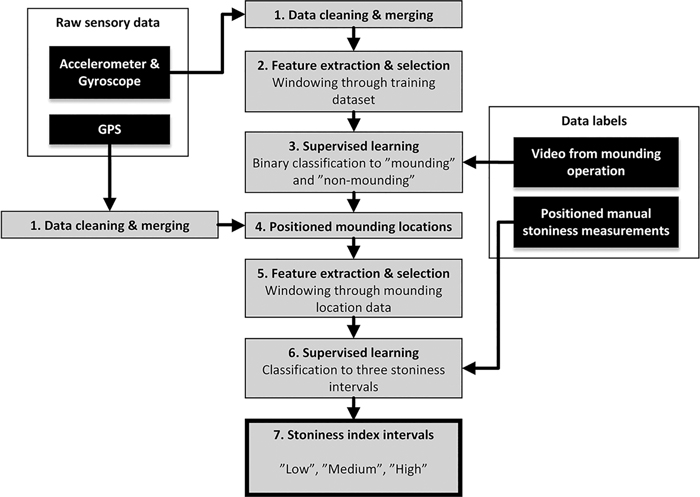
Fig. 1. Stoniness classification process of forest soil, based on the excavator IMU data.
2.1 Data collection setup
The collected data consists of the vibration measurements from the excavator boom, the GPS location and manual stoniness measurements of the mounded forest ground. The excavator was a Doosan DX140LCR crawler (Doosan 2019), weighing approximately 15 tonnes. The attached mounding blade had a width of 52 centimeters. The automatic measurements were collected from four separate mounding sites in the Valkeakoski region in southern Finland during November and December 2017. These measurements were gathered during a normal mounding operation, and thus represent true forest operation conditions. The logging residues from the clear-cutting had been removed from the site before the measurements were taken, but the stumps had been left in place, which is common practice before spot-mounding. The temperature during the data collection period fluctuated around zero degrees, but the ground was free from snow and frost. The soil types in the area consisted of sandy moraine, fine sandy moraine and silty moraine.
The vibrations of the excavator boom were measured using a special-purpose measurement device that was attached to the boom near the mounding blade (Fig. 2). The measurement device consisted of an IMU, a GPS receiver, a small computer for storing the measurements and a battery. The IMU was an Adafruit BNO055, which is based on a Bosch BNO055 9-axis absolute orientation sensor (Bosch Sensortec 2014). This sensor consists of an accelerometer, a gyroscope and a magnetometer, each having three axes, and it is capable of fusing the measurements together in real time before sending them to the data acquisition computer. The measurement axes of the IMU are marked in Fig. 2. The GPS receiver was a Haicom HI-204III-USB GPS receiver (Haicom 2018). The IMU is capable of producing linear acceleration output by preprocessing the accelerometer data using internal data-fusion algorithms. This study utilizes the fused linear acceleration and raw gyroscope measurements. The IMU measurements were gathered at a sampling frequency of 100Hz and the GPS locations were updated every second.
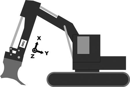
Fig. 2. A drawing of the measurement setup and the coordinate axes in the excavator. The location of the measurement device is marked with the “IMU” label (IMU = inertial measurement unit).
In addition to the automatic vibration measurements, manual measurements were collected after the mounding work was completed for each site. The manual measurements were performed according to the method suggested by Viro (1952). This is a straightforward method for obtaining a single stoniness index measurement. A sharp steel bar with a diameter of 12 mm was inserted into the ground to a depth of 20 centimeters and the number of hit stones was recorded. In this study, each stoniness index measurement consisted of ten penetrations in a straight line at intervals of one meter. The percentage of hit stones within the penetrations gives the stoniness index in the center of the measurement line. This procedure thus returned stoniness indices at percentages of from 0to 100% at intervals of 10%. The direction of the measurement line was selected according to the assumed route of the excavator, ensuring that the measurements were only taken from the same locations as where the IMU had recorded the excavator boom vibrations. Fig. 3 shows the locations of the measured stoniness indices at the four sites, each produced with ten penetrations. The initial manual measurements were conducted in November 2017, under much the same conditions as for the IMU measurements. The ground was fairly wet as it had rained for several days at the end of October, but the temperature was fluctuating around zero and there was no snow or frost. The manual measurements were divided into three stoniness classes as suggested by Viro (1952) in the following manner: 0to 30% for low stoniness, 40 to 60% for medium stoniness and 70 to 100% for high stoniness.
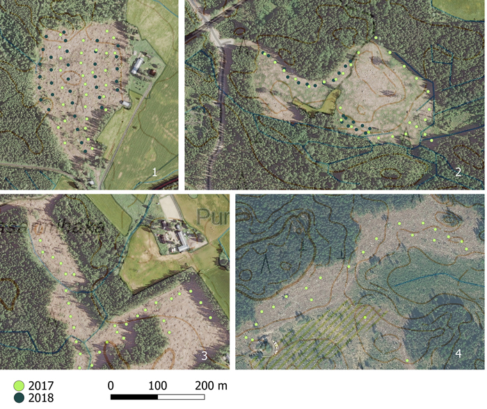
Fig. 3. Manual stoniness measurements at four different sites. The circles are the center points for the series of 10 bar insertions and the color indicates the year of the measurements. (Aerial photo © National Land Survey of Finland 2018).
The convention of measuring the index along a line in single direction introduces a degree of uncertainty for the manual measurements and consequently to the ground truth of the automatic classification process. In order to evaluate the accuracy of the manual measurements and to validate the predictive models, another set of manual measurements were taken from sites 1 and 2 in August 2018 (Fig. 3). These later manual measurements were performed at the sites where the variability of the stoniness index seemed to be highest in the earlier measurements. The weather conditions were completely different from the initial measurements taken the previous autumn, as the summer of 2018 was dry in Finland, although the weather should not significantly affect the manual stoniness index measurement process.
2.2 Activity recognition
The development of an excavator-activity recognition algorithm was done with the aid of a video recording of the mounding work. This video consists of approximately 10 minutes of the mounding work and it included a total of 46 mounding movements. The excavator was halted in order to synchronize the video and sensor times. Based on the video, segments of the IMU data were labeled manually as being either mounding or non-mounding operations. With this training set, the machine-learning classifiers were trained to detect the digging phase in the mounding motion sequence based on the IMU data alone.
The first step in the activity recognition process was to extract the relevant features from the IMU signals. A window of 400 measurements, meaning a duration of 4 seconds, was employed for this purpose. This window length is justified by the fact that the average length of a digging motion in the labeled data was 3.5 seconds. The data windows were overlapped by 50% (200 measurements), as this procedure has been found to be efficient in other activity recognition studies (Akhavian and Behzadan 2015; Gupta and Dallas 2014). A set of features was calculated over each window in each sensor axis. The features were initially selected based on other researchers’ experience in handling similar problems in the literature (Akhavian and Behzadan 2015; Gupta and Dallas 2014; Liu et al. 2012). The selected initial features are listed in Table 1.
| Table 1. Initial features before feature selection. | ||
| Features for IMU signals | ||
| Basic descriptive statistics | Mean | Minimum |
| Median | Maximum | |
| Standard deviation (STD) | 25th percentile | |
| Variance | 75th percentile | |
| Median absolute deviation (MAD) | Skewness | |
| Interquartile range (IQR) | Kurtosis | |
| Signal metrics | Peak to peak | |
| Root-mean-square level (RMS) | ||
| Signal power | ||
| 1-lag autocorrelation | ||
| Frequency domain properties | Dominant frequency | |
| Dominant frequency magnitude | ||
| Correlations | Correlation coefficients between axes | |
A total of 123 different features were calculated (108 single signal features and 15 correlations) as there were six measurement axes (three in the accelerometer and three in the gyroscope). The feature space is very large compared to the available training data, so the established practice is to whittle the feature space down until it only contains the most relevant features. Two feature selection algorithms, ReliefF (MathWorks 2018b), and Sequential feature selection (MathWorks 2018c) in Matlab, were used to select the most appropriate features. A sequential feature selection (SFS) algorithm was performed 5 times for each model and any individual features that appeared in more than one of the selections were chosen as final features. The ReliefF algorithm ranks the features according to their importance, so the final number of features was determined by observing which number of the ranked features minimizes the misclassification rate in the cross-validation process. The algorithms can select very different features for training, so the performance of the classifiers is reported using both approaches.
In this study, the following supervised learning classifiers were trained: Support Vector Machine (SVM), Binary Decision Tree (BDTree), NaïveBayes, Linear Discriminant Analysis (LDA), Quadratic Discriminant Analysis (QDA), K-Nearest Neighbors (KNN) and a neural network model (ANN). Each of the models were trained using uniquely selected features, except for the neural network model, which was trained using all 123 features as a point of comparison. The ANN model was a feed-forward network consisting of one hidden layer with 10 nodes. The accuracy of each trained classifier was evaluated using 10-fold cross-validation, which divides the dataset into 10 folds and uses each fold in turn for testing while the other folds are used for training. The result of the classification is applied in selecting the data for the stoniness classifications, so the models can be trained by assigning a higher cost for a false positive classification. Although this results in lower overall accuracy, it tends to leave more data out of the second phase rather than including data that was not generated by the digging activity. For example, the cost of a false-positive classification can be set twice as high as the cost of a true-positive classification in the cost matrix given for the algorithm. The final activity recognition models were trained using all the available data and the best performing model was defined using the averaged accuracy of the cross-validation.
2.3 Stoniness classification
The stoniness classification process starts by detecting the digging periods from all the recorded IMU data using the best-performing activity recognition model. Only those parts of the data classified as “digging” are utilized in the stoniness classification, so any vibrational data that did not originate from the mounding blade’s contact with the soil is ignored. This process also selects data that has been falsely classified as digging by the first classifier, but the errors can be minimized by applying higher classification costs for the false-positive classifications, as described in the previous section. The resulting dataset for all the measured data consisted of approximately 70 000 data windows.
The stoniness class labels for the supervised learning setting are based on the manual measurements. Since the manual measurements were pointwise and did not cover the whole measured site, the manual measurements that were within a radius of four meters from the mounding locations were used for labeling. Of the 70 000 data windows, approximately 3000 were labelled with manual measurements. Only the labeled parts of the IMU data could be used for training the model and for the final accuracy evaluation of the predicted stoniness classes.
The stoniness classification process was evaluated using the same classifier algorithms as for the activity recognition, but multiclass versions (MathWorks 2018a) of them were needed to predict three classes instead of two. The features for the IMU signals were calculated again for the mounding windows. The initial features were the same as in the activity recognition, but the feature selection algorithms (ReliefF and SFS) utilized the stoniness class labels and selected different features to be calculated. This labeled dataset, approximately 3000 observations, was 10-fold cross-validated to evaluate the accuracy of the stoniness classifications. After the accuracy estimation, the classification models were again trained using all the labeled data, and the stoniness classes of the unlabeled dataset was predicted using all the models.
The output of a stoniness classification model is a probability distribution for the three stoniness classes (low, medium, high) for each mounding point, i.e. three probabilities, totaling one in all, for every soil contact period in the data. The stoniness class with the highest probability is chosen as the predicted class for the mounding point.
2.4 Grid representation
The classification model of the stoniness index returns the stoniness class predictions, hereafter called point predictions, for each window of data. A single digging motion could produce more than one prediction for the stoniness class due to the windowing of the data. Furthermore, the generated mounds are not evenly distributed over the forest site, so a robust representation of the data is needed to generate useful databases for the stoniness information. In this study, the previously-mentioned grid of 16 × 16 m cells is utilized for aggregating such data points into a map with regular intervals for the stoniness classes. In the collected data, one cell typically contains 10 to 150 predictions of the stoniness class. The most frequent prediction (i.e. the mode) of the single-mound predictions inside the grid cell was selected as the stoniness class of the cell in question (hereafter called grid prediction).
The grid prediction gives more coarse information about the soil stoniness in the forest sites than the individual point predictions, but it is also more comparable to the resolution of the manual measurement technique that was used. For this reason, a heuristic accuracy measure was calculated using the grid cell neighborhood of each manual measurement. In other words, each manual measurement was examined together with four of the nearest grid cell predictions. A correctly classified prediction was recorded if the nearest cell prediction agreed with the manual measurement, or if at least 50% of the four nearest grid cell predictions agreed with the manual measurement class. The grid prediction was cross-validated in the same manner as the point prediction.
Moreover, an entropy measure was calculated based on the predicted stoniness classes inside each cell. Entropy, according to information theory, describes the average lack of information contained in an observation, i.e. the uncertainty of a discrete-valued random variable (here the cell stoniness class). High entropy means low predictability. The entropy for the single cell k is defined as:

where m is the number of different predicted classes (here three), ni is the summed occurrence of i:th class inside the cell and N is the total number of predictions inside the cell. If all classes occur with the same frequency, the entropy is at its highest, 1.585. If, for example, two classes are equally frequent and the third does not occur at all, the entropy is 1. Both the final grid cell prediction and the entropy are dependent on the performance of the classification model. They are reported only for the model that shows the best results when compared to the manual measurements. Single grid cells contain different numbers of predictions in this study, and some grid cells have only a few measurements. In this study, grid cells having less than 10 predictions were not regarded as representative samples of the variability of the stoniness inside the cell, so a threshold of 10 predictions was used to exclude these cells from the entropy evaluation.
3 Results
3.1 Feature selection
The features ranked most important by the ReliefF algorithm are presented in Table 2. Only the 25 most important features are listed. The features were individually selected for each classification model based on the combination that best minimizes the classification error. Fig. 4 shows the 10-fold cross-validated misclassification rate with different numbers of features taken from the ReliefF algorithm feature-ranking results. Fig. 4a shows the error progression in the first classification task (activity recognition) and Fig. 4b, in the second classification task (stoniness classification).
| Table 2. Features ranked highest by the ReliefF algorithm. | ||
| Ranked features for each axis by the ReliefF algorithm (Rank order) | ||
| Activity recognition | Stoniness classification | |
| Accelerometer X | - | Minimum (10) Maximum (18) Peak to peak (20) Dominant frequency magnitude (21) Autocorrelation (22) |
| Accelerometer Y | Kurtosis (4) Maximum (5) MAD (11) IQR (14) 75-percentile (24) | Max (2) Peak to peak (3) Autocorrelation (5) 75-percentile (12) STD (14) Minimum (16) Dominant frequency (23) Power (24) Variance (25) |
| Accelerometer Z | Dominant frequency magnitude (7) Autocorrelation (12) Mean (15) 75-percentile (22) Median (25) | Autocorrelation (13) MAD (15) IQR (19) |
| Gyroscope X | MAD (1) Dominant frequency magnitude (10) 75-percentile (21) | Autocorrelation (6) |
| Gyroscope Y | - | Autocorrelation (8) |
| Gyroscope Z | Minimum (3) 75-percentile (6) Median (8) 25-percentile (13) Mean (20) MAD (23) | - |
| Correlation coeff. | Acc. X – Acc. Y (2) Acc. Y – Acc. Z (9) Gyro. Y – Gyro. Z (19) | Gyro. X – Gyro. Y (1) Acc. Z – Gyro. Y (4) Acc. X – Acc. Y (7) Acc. Y – Gyro. X (9) Acc. Z – Gyro. X (11) Acc. X – Gyro. Z (17) |
| STD = standard deviation, MAD = Median absolute deviation, IQR = Interquartile range. | ||
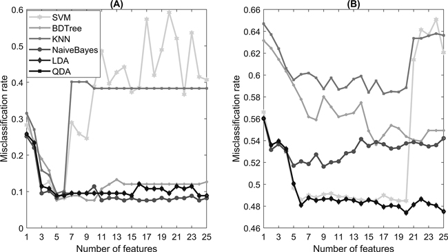
Fig. 4. The misclassification rate with an increasing number of features selected by the ReliefF algorithm in (A) activity recognition and (B) stoniness classification.
In the activity recognition task, most of the models have only small variations in the misclassification rate after five selected features. However, the SVM and KNN models show significantly worse prediction results when the number of selected features is increased. This same behavior due to overfitting is somewhat visible in the stoniness classification task.
The SFS algorithm selected the features directly using the 10-fold cross-validation and the misclassification rate. The selected features for the activity recognition are listed in Table 3 and for the stoniness classification in Table 4. The number of the selected features is similar to the results presented with the ReliefF algorithm in Fig. 4, but the selected features themselves are actually different.
| Table 3. Selected features in activity recognition by the SFS algorithm. | ||||||
| Selected features for each axis by the SFS algorithm (activity recognition) | ||||||
| SVM | BDTree | KNN | NaïveBayes | LDA | QDA | |
| Accelerometer X | RMS Peak to peak | Minimum | - | - | - | - |
| Accelerometer Y | Variance | STD | Maximum STD Peak to peak | STD | Variance | Variance |
| Accelerometer Z | - | - | - | - | - | - |
| Gyroscope X | - | - | 25-percentile | Median | MAD | MAD |
| Gyroscope Y | - | Peak to peak | - | - | - | - |
| Gyroscope Z | - | - | - | Mean | Mean | Mean |
| SVM = Support Vector Machine, BDTree = Binary Decision Tree, KNN = K-Nearest Neighbors, LDA = Linear Discriminant Analysis, QDA = Quadratic Discriminant Analysis. RMS = Root-mean-square level, STD = standard deviation, MAD = Median absolute deviation. | ||||||
| Table 4. Selected features in stoniness classification by the SFS algorithm. | ||||||
| Selected features for each axis by the SFS algorithm (stoniness classification) | ||||||
| SVM | BDTree | KNN | NaïveBayes | LDA | QDA | |
| Accelerometer X | Dom. freq. | - | - | - | RMS 75-percentile Dom. freq. mag. | RMS 75-percentile Dom. freq. mag. |
| Accelerometer Y | Autocorrelation | - | - | Mean Skewness Autocorrelation | Median Maximum Variance Power Autocorrelation | Median Maximum Variance Power Autocorrelation |
| Accelerometer Z | STD 75-percentile | - | - | Median 75-percentile | Mean | Mean |
| Gyroscope X | Maximum | - | - | - | Maximum Peak to peak | Maximum Peak to peak |
| Gyroscope Y | Maximum | - | - | MAD | MAD Kurtosis Peak to peak | MAD Kurtosis Peak to peak |
| Gyroscope Z | Minimum | Dom. freq. | Dom. freq. | - | Minimum Autocorrelation | Minimum Autocorrelation |
| Correlation coeff. | - | - | - | Acc. X – Acc. Y Acc. X – Gyro. Y | Acc. X – Gyro. Y | Acc. X – Gyro. Y |
| SVM = Support Vector Machine, BDTree = Binary Decision Tree, KNN = K-Nearest Neighbors, LDA = Linear Discriminant Analysis, QDA = Quadratic Discriminant Analysis. RMS = Root-mean-square level, STD = standard deviation, MAD = Median absolute deviation. | ||||||
3.2 Activity recognition
The average accuracy calculated using the 10-fold cross-validation for the activity recognition is presented in Fig. 5. The figure shows also the percentage of false-positive predictions, which are harmful for the subsequent stoniness classification.
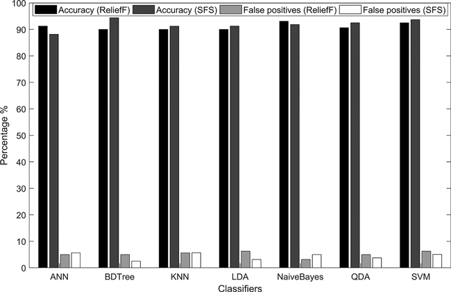
Fig. 5. The accuracy and percentage of false-positive predictions in the activity recognition using two feature-selection algorithms, ReliefF and Sequential Feature Selection (SFS).
Based on the results, the BDTree classifier with features selected by the SFS algorithm was chosen as the best model for activity recognition as it had an accuracy of 94.4%. The model in question predicted an average 2.5% of the labels as false positives. Essentially, all the models gave uniform results that showed an averaged accuracy of near 90%.
3.3 Stoniness prediction
The cross-validated accuracy of the stoniness prediction is presented in Table 5. The accuracies for the point predictions are rather low, due to the fact that the labels were generalized for a larger group of predicted points from a single manual measurement. Table 5 also shows the grid prediction accuracy, which better describes the success of the classification within the grid cell resolution. The grid prediction accuracy is calculated for the second set of manual measurements.
| Table 5. The stoniness prediction accuracy. | |||||||
| Stoniness prediction accuracy (%) | |||||||
| SVM | BDTree | KNN | NaïveBayes | LDA | QDA | ANN | |
| Point prediction (ReliefF) | 43.3 | 43.8 | 42.6 | 42.6 | 47.6 | 44.6 | 43.0 |
| Point prediction (SFS) | 45.0 | 37.7 | 45.6 | 44.6 | 44.6 | 40.8 | 43.0 |
| Grid prediction (ReliefF) | 66.1 | 69.6 | 37.5 | 64.3 | 35.7 | 57.1 | 62.5 |
| Grid prediction (SFS) | 75.0 | 26.8 | 46.4 | 50.0 | 28.6 | 53.6 | 62.5 |
| SVM = Support Vector Machine, BDTree = Binary Decision Tree, KNN = K-Nearest Neighbors, LDA = Linear Discriminant Analysis, QDA = Quadratic Discriminant Analysis, ANN = a neural network model. | |||||||
Figs. 6–9 show the predicted stoniness classes for each measured site individually. The prediction results are accumulated in the grid cells as described in the Materials and Methods section. In the figures, the area formed by the predicted grid cells is the site where the excavator was moving, in other words the locations where the IMU measurements were recorded. The manually-measured stoniness classes are laid on top of the predicted grid cells to give a good visualisation of the prediction performance.
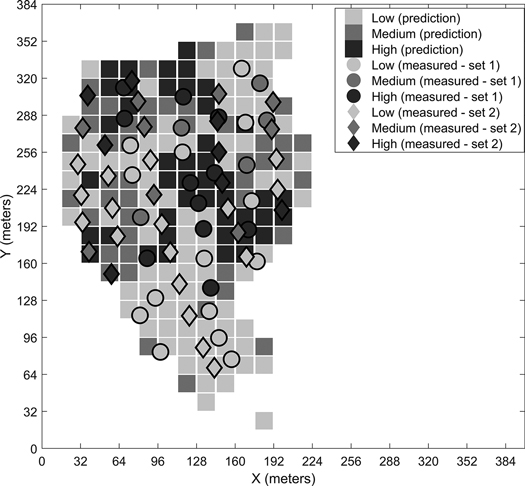
Fig. 6. Predicted stoniness classes and manual measurements for the first site.
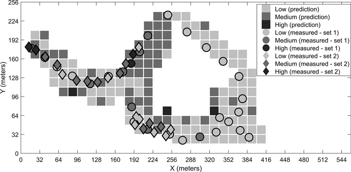
Fig. 7. Predicted stoniness classes and manual measurements for the second site.
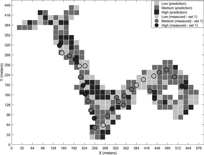
Fig. 8. Predicted stoniness classes and manual measurements for the third site.
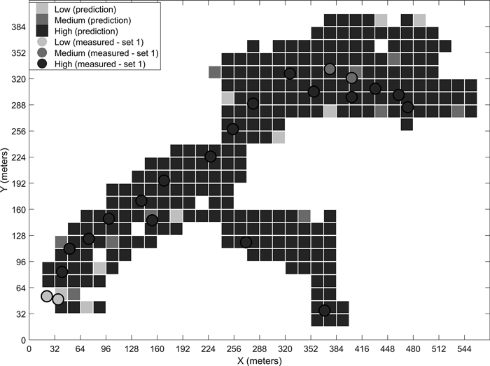
Fig. 9. Predicted stoniness classes and manual measurements for the fourth site.
3.4 Entropy of the stoniness prediction
The calculated entropy for the grid cells is presented in Fig. 10 for the first site. Calculation of the cell entropies for the other sites returned similar results. A large entropy value (near the maximum value of 1.585) for a grid cell suggests that all three of the stoniness classes are evenly predicted inside the grid cell. This implies a large variation of the stoniness inside the grid cell, and consequently the predicted class would not have much use for forestry applications.
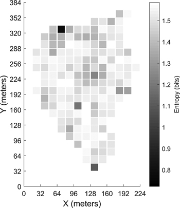
Fig. 10. Entropy calculated for each grid cell in the first site.
4 Discussion
Knowledge of the prevailing forest soil stoniness is an asset when planning forestry operations, but it is not usually available before actually visiting the site. Therefore, we present a solution for automatically classifying soil stoniness during mounding work. This method of classification only needs an IMU and a GPS receiver and thus enables an affordable solution for the problem, as these devices have already been commercially developed for use with heavy machinery, such as excavators. As this data about the stoniness of the soil is not gathered until the mounding work is done, we cannot directly improve the soil preparation process with these measurements. However, the main idea is to gradually build up an exhaustive database that could be utilized in subsequent forest operation phases and could act as a reference for new stoniness models and measurement methods. These are currently needed in Finland as there is an upcoming project for closely mapping the soil properties of the whole country. In this project, novel models are being developed for estimating soil stoniness which, for instance, fuse available but heterogeneous data sources, such as remotely-sensed and manually-collected soil data. In this respect, our automatically-collected reference data for soil stoniness would be extremely useful in building generalizable stoniness models for larger geographic areas. In addition, the recorded stoniness information can aid subsequent phases in the forest renewal process, such as planting (Lideskog et al. 2014) and harvesting. Furthermore, as the physical properties of the soil are strongly influenced by its stoniness (Eriksson and Holmgren 1996; Stendahl et al. 2009), hydrology models could be improved if the stoniness is already known. Hydrology models are utilized, for example, to make estimations of the forest’s trafficability (Salmivaara et al. 2017), so improved hydrology models could be very useful in planning thinning operations in the future. As areas for further study, larger training sets are needed to cover the effects of different mounding site conditions, different types of excavator and possible differences in the behavior of different excavator operators.
This paper has proposed an automated two-stage procedure for classifying the stoniness of forest soil into three categories. One of the first results of this study is a procedure for selecting suitable features from the IMU signals and for deciding what windowing procedures should be applied. Although we did not report the results obtained with other window lengths here, no significant improvements were observed with window sizes of 100, 200 or even 600 samples, so it can be said that the selected window lengths seem to work well. We performed the feature selection using two different algorithms to reduce the risk of drawing false conclusions about the selected features. The results for the activity recognition shows that the selected features clearly differ between the selection algorithms. However, both of the methods selected many features from the Y-axis of the accelerometer (Table 2 and Table 3), so we have assumed it to be the most important axis for recognizing any digging motion. This was as expected because the Y-axis is parallel with the direction of the digging motion. Therefore, the mounding blade’s contact with the soil is likely to cause vibrations on the excavator boom in the Y direction. We also expected the gyroscope measurements to be important in distinguishing the occasions when the machine is not digging, as the gyroscope easily detects the rotation of the excavator boom. The same reasoning applies for the stoniness classification, the Y- and X-axes of the accelerometer are expected to sense the vibrations caused by different soil stoniness levels.
The classification of the excavator activities into “digging” and “non-digging” is essential for detecting relevant data for the stoniness classification. In this context, it is important to be able to detect the most certain digging motions, as activities incorrectly labelled as “digging” would result in predicting the stoniness class of the soil from data that was not produced from contact with the soil. For this reason, the activity classifiers should be trained so that false-positive results are more costly than false negative results. Furthermore, on the whole the number of predictions per grid cell is pretty high, so mistakenly discarding data from the stoniness classification is not an issue. We found the activity recognition results to be consistent using both feature-selection algorithms and with all the supervised learning algorithms. This suggests that the digging motion has been correctly detected, and therefore the first classification task is justified. Nevertheless, the dataset for the activity detection was relatively small, so all the possible mounding conditions have probably not yet been covered.
In the stoniness classification process, the low number of manual measurements did not yield enough training data for the classifier training. For this reason, we used a radius of four meters around the center point of the manual measurement to label the detected mounding locations according to their class. This was a coarse generalization, which surely does not represent the true variation in the soil’s stoniness. However, the required resolution in the final application is probably in the region of 16 × 16 meter cells, which is the resolution used by many forest operation planning systems in Finland. Consequently, the generalization of the manual measurements is reasonable, but it does result in seemingly poor accuracy results if calculated for each single predicted data point. In addition, the point accuracy does not seem to describe the large differences that are evident when visually inspecting the stoniness predictions by the different classifiers. The accuracy we calculated for the grid prediction provides a more meaningful evaluation of the accuracy as it arranges the classifiers in the order that agrees with human reasoning. Nonetheless, due to the measurement procedure of measuring along a line in one direction, repeated manual measurements inside the grid cell can have notable variations. The uncertainty of the manual measurements is seemingly the most significant error source in the model training and evaluation. For practical reasons, the manual and automatic measurements rely on different GPS devices, which may result in misalignment of the measurements when comparing them to each other, although we consider this error source to be negligible.
We have presented the predicted results for the four different sites for the best-performing classifier. The visual examination of the predicted grids and the manual measurements together give an idea of the classifiers’ performances. For example, in the prediction map of the third site (Fig. 8), the few locations where low stoniness was detected in the manual measurements were also estimated as low stoniness in the final prediction. If we compare the sites with generally low or high stoniness, i.e. the second and fourth sites, the classifier predicts the results logically according to the dominant class. These observations suggest that the model is capable of detecting different stoniness classes and has not overfitted to a certain condition. Furthermore, we did not observe any notable differences in the prediction accuracies for single classes, i.e. the reported overall accuracy describes the predictability of all three classes well.
In any final application of this methodology, the excavator would record the data, and perform the soil stoniness classification with a pre-trained classification model. As seen from the presented entropy map (Fig. 10), the uncertainty of the classification varies and the amount of single predictions per grid can be quite different. Therefore, the entropy of a single grid cell could be used to evaluate whether the predicted class is a representative estimate for the whole grid cell. The degree of entropy needs to be taken into account when saving the predicted classes to a database, and probably some thresholds for separating uncertain predictions from the reliable ones are needed. The entropy value can give misleading interpretations for the variability of the stoniness in the grid cell if it is calculated using only a few point predictions. In this study, we have excluded some of the grids from the entropy analysis using an arbitrarily selected threshold of 10 point predictions. We do not suggest here that this is an optimal threshold value, but such a value could be assessed when more measurement data is available. In addition to the grid cell entropy, the probability distribution of a single point prediction could be used to determine whether the point is taken into account when calculating the grid cell prediction.
In conclusion, the results show that the three-class stoniness classification has an accuracy of up to 70% when using a moderate spatial resolution for the predictions, such as the 16 × 16 m cell grid. In addition, with our test data the detection of the digging motion achieved over 90% accuracy. These results suggest that equipping excavators used in soil preparation operations with inexpensive inertial measurement units would facilitate the collection of comprehensive information about the stone content of the upper layers of forest soil. Further research is needed to investigate whether other sensors, such as pressure sensors for the hydraulic cylinders of the excavator, could be utilized to further develop the classification accuracy, and larger datasets are needed to cover different field conditions. However, it has been shown that it is possible to automatically collect information about soil stoniness during forest mounding operations with only minor changes to the mounding machinery. This could eventually lead to more efficient (and economical) forestry operations and would also produce valuable reference data for developing more extensive soil models.
References
Äijälä O., Koistinen A., Sved J., Vanhatalo K., Väisänen P. (2014). Metsänhoidon suositukset [Forest management recommendations]. Metsätalouden kehittämiskeskus Tapion julkaisuja. [In Finnish].
Akhavian R., Behzadan A.H. (2015). Construction equipment activity recognition for simulation input modeling using mobile sensors and machine learning classifiers. Advanced Engineering Informatics 29(4): 867–77. https://doi.org/10.1016/J.AEI.2015.03.001.
Alexander E.B. (1981). Volume estimates of coarse fragments in soils: a combination of visual and weighing procedures. Journal of Soil and Water Conservation 36(6): 360–61.
Baritz R., Seufert G., Montanarella L., Van Ranst E. (2010). Carbon concentrations and stocks in forest soils of Europe. Forest Ecology and Management 260(3): 262–77. https://doi.org/10.1016/j.foreco.2010.03.025.
Bosch Sensortec (2014). BNO055 intelligent 9-axis absolute orientation sensor. https://cdn-shop.adafruit.com/datasheets/BST_BNO055_DS000_12.pdf.
Botero Valencia J.-S., Rico Garcia M., Villegas Ceballos J.-P. (2017). A simple method to estimate the trajectory of a low cost mobile robotic platform using an IMU. International Journal on Interactive Design and Manufacturing (IJIDeM) 11(4): 823–28. https://doi.org/10.1007/s12008-016-0340-5.
Coppola A., Dragonetti G., Comegna A., Lamaddalena N., Caushi B., Haikal M.A., Basile A. (2013). Measuring and modeling water content in stony soils. Soil and Tillage Research 128: 9–22. https://doi.org/10.1016/j.still.2012.10.006.
Doosan (2019). Doosan DX140LCR brochure. http://www.doosanequipment.com/assets/imported/transformations/content/product-details/%7Blanguage%7D_Brochure/E69F10C046AE492CB0BF42197A66DBC2/Crawler-Excavators-DX140LC-5-DX255LC-5-14-28-metric-ton.PDF.
Dzerina B., Girdziusas S., Lazdina D., Lazdins A., Jansons J., Neimane U., Jansons Ā. (2016). Influence of spot mounding on height growth and tending of Norway spruce: case study in Latvia. Forestry Studies. Metsanduslikud Uurimused 65: 24–33.
Eriksson C.P., Holmgren P. (1996). Estimating stone and boulder content in forest soils – evaluating the potential of surface penetration methods. Catena 28(1–2): 121–34. https://doi.org/10.1016/S0341-8162(96)00031-8.
Fardusi M.J., Chianucci F., Barbati A. (2017). Concept to practices of geospatial information tools to assist forest management & planning under precision forestry framework: a review. Annals of Silvicultural Research 41(1): 3–14. https://doi.org/10.12899/asr-1354.
Gupta P.P., Dallas T. (2014). Feature selection and activity recognition system using a single triaxial accelerometer. IEEE Transactions On Biomedical Engineering 61(6): 1780–86. https://doi.org/10.1109/TBME.2014.2307069.
Haicom (2018). HI-204III USB GPS receiver datasheet. http://www.haicom.com.tw/GPS_Receivers/HI-204IIIUSB/Product.aspx.
Hammerla N.Y., Halloran S., Ploetz T. (2016). Deep, convolutional, and recurrent models for human activity recognition using wearables. ArXiv Preprint 1604.08880.
Hauglin M., Hofstad Hansen E., Næsset E., Even Busterud B., Omholt Gjevestad G.J., Gobakken T. (2017). Accurate single-tree positions from a harvester: a test of two global satellite-based positioning systems. Scandinavian Journal of Forest Research 32(8): 774–781. https://doi.org/10.1080/02827581.2017.1296967.
Holopainen M. (2011). Effect of airborne laser scanning accuracy on forest stock and yield estimates. Aalto University Doctoral Dissertations 6/2011. Aalto University, School of Engineering, Department of Surveying. https://aaltodoc.aalto.fi/handle/123456789/4912.
Holopainen M., Vastaranta M., Hyyppä J. (2014). Outlook for the next generation’s precision forestry in Finland. Forests 5(7): 1682–94. https://doi.org/10.3390/f5071682.
Karlsson K. (2000). Height growth patterns of Scots pine and Norway spruce in the coastal areas of western Finland. Forest Ecology and Management 135(1–3): 205–216. https://doi.org/10.1016/S0378-1127(00)00311-X.
Lideskog H., Ersson B.T., Bergsten U., Karlberg M. (2014). Determining boreal clearcut object properties and characteristics for identification purposes. Silva Fennica 48(3) article 1136. https://doi.org/10.14214/sf.1136.
Lindroos O., Ringdahl O., La Hera P., Hohnloser P., Hellström T. (2015). Estimating the position of the harvester head – a key step towards the precision forestry of the future? Croatian Journal of Forest Engineering 36(2): 147–64.
Liu S., Gao R., Freedson P. (2012). Computational methods for estimating energy expenditure in human physical activities. Medicine & Science in Sports & Exercise 44(11): 2138–46. https://doi.org/10.1249/MSS.0b013e31825e825a.
Löf M., Dey D.C., Navarro R.M., Jacobs D.F. (2012). Mechanical site preparation for forest restoration. New Forests 43(5–6): 825–48. https://doi.org/10.1007/s11056-012-9332-x.
Löf M., Ersson B.T., Hjältén J., Nordfjell T., Oliet J.A., Willoughby I. (2015). Site preparation techniques for forest restoration. In: Stanturf J.A. (ed.). Restoration of boreal and temperate forests. p. 85–102. CRC Press.
Londo A.J., Mroz G.D. (2001). Bucket mounding as a mechanical site preparation technique in wetlands. Northern Journal of Applied Forestry 18(1): 7–13.
Luoranen J., Saksa T., Finér L., Tamminen P. (2007). Metsämaan muokkausopas. Metsäntutkimuslaitos, Suonenjoki. [In Finnish]. http://urn.fi/URN:ISBN:978-951-40-2059-9.
MathWorks (2018a). Fit multiclass models. https://se.mathworks.com/help/stats/fitcecoc.html.
MathWorks (2018b). ReliefF algorithm. https://se.mathworks.com/help/stats/relieff.html.
MathWorks (2018c). Sequential feature selection. https://se.mathworks.com/help/stats/sequentialfs.html.
Melander L., Ritala R. (2018). Time-of-flight imaging for assessing soil deformations and improving forestry vehicle tracking accuracy. International Journal of Forest Engineering 29(2): 63–73. https://doi.org/10.1080/14942119.2018.1421341.
Menna B.V., Villar S.A., Rozenfeld A., Acosta G.G. (2017). GPS aided strapdown inertial navigation system for autonomous robotics applications. 2017 XVII Workshop on Information Processing and Control (RPIC). 6 p. https://doi.org/10.23919/RPIC.2017.8211625.
Nevalainen P., Middleton M., Sutinen R., Heikkonen J., Pahikkala T. (2016). Detecting terrain stoniness from Airborne Laser Scanning data. Remote Sensing 8(9): 1–21. https://doi.org/10.3390/rs8090720.
Olivera A., Visser R., Acuna M., Morgenroth J. (2016). Automatic GNSS-enabled harvester data collection as a tool to evaluate factors affecting harvester productivity in a Eucalyptus spp. harvesting operation in Uruguay. International Journal of Forest Engineering 27(1): 15–28. https://doi.org/10.1080/14942119.2015.1099775.
Panagos P., Meusburger K., Ballabio C., Borrelli P., Alewell C. (2014). Soil erodibility in Europe: a high-resolution dataset based on LUCAS. Science of the Total Environment 479–480(1): 189–200. https://doi.org/10.1016/j.scitotenv.2014.02.010.
Pavey T.G., Gilson N.D., Gomersall S.R., Clark B., Trost S.G. (2017). Field evaluation of a random forest activity classifier for wrist-worn accelerometer data. Journal of Science and Medicine in Sport 20(1): 75–80. https://doi.org/10.1016/j.jsams.2016.06.003.
Rantala J., Saarinen V.-M., Hallongren H. (2010). Quality, productivity and costs of spot mounding after slash and stump removal. Scandinavian Journal of Forest Research 25(6): 507–14. https://doi.org/10.1080/02827581.2010.522591.
Saarinen V.-M. (2006). The effects of slash and stump removal on productivity and quality of forest regeneration operations – preliminary results. Biomass and Bioenergy 30(4): 349–56. https://doi.org/10.1016/j.biombioe.2005.07.014.
Sabato A., Niezrecki C., Fortino G. (2017). Wireless MEMS-based accelerometer sensor boards for structural vibration monitoring: a review. IEEE Sensors Journal 17(2): 226–35. https://doi.org/10.1109/JSEN.2016.2630008.
Saksa T., Miina J., Haatainen H., Kärkkäinen K. (2018). Quality of spot mounding performed by continuously advancing mounders. Silva Fennica 52(2) article 9933. https://doi.org/10.14214/sf.9933.
Salmivaara A., Launiainen S., Ala-Ilomäki J., Kulju S., Laurén A., Sirén M., Tuominen S., Finér L., Uusitalo J., Nevalainen P., Pahikkala T., Heikkonen J. (2017). Dynamic forest trafficability prediction by fusion of open data, hydrologic forecasts and harvester-measured data. Young Researchers Challenge 2017, Stockholm. Poster. http://urn.fi/URN:NBN:fi-fe2017102450272.
Salmivaara A. Miettinen M., Finér L., Launiainen S., Korpunen H., Tuominen S., Jukka Heikkonen, Nevalainen P., Sirén M., Ala-Ilomäki J., Uusitalo J. (2018). Wheel rut measurements by forest machine-mounted LiDAR sensors – accuracy and potential for operational applications? International Journal of Forest Engineering 29(1): 1–12. https://doi.org/10.1080/14942119.2018.1419677.
Singleton R.K, Strangas E.G., Aviyente S. (2017). The use of bearing currents and vibrations in lifetime estimation of bearings. IEEE Transactions on Industrial Informatics 13(3): 1301–1309. https://doi.org/10.1109/TII.2016.2643693.
Stendahl J., Lundin L., Nilsson T. (2009). The stone and boulder content of swedish forest soils. Catena 77(3): 285–91. https://doi.org/10.1016/j.catena.2009.02.011.
Sutton R.F. (1993). Mounding site preparation: a review of European and North American experience. New Forests 7(2): 151–92. https://doi.org/10.1007/BF00034198.
Trost S.G., Zheng Y., Wong W.K. (2014). Machine learning for activity recognition: hip versus wrist data. Physiological Measurement 35(11): 2183–2189. https://doi.org/10.1088/0967-3334/35/11/2183.
Viro P.J. (1952). On the determination of stoniness. Communicationes Instituti Forestalis Fenniae 40,3. 23 p. http://urn.fi/URN:NBN:fi-metla-201207171072.
White J.C., Wulder M.A., Varhola A., Vastaranta M., Coops N.C., Cook B.D., Pitt D., Woods M. (2013). A best practices guide for generating forest inventory attributes from airborne laser scanning data using an area-based approach. Forestry Chronicle 89(6): 722–23. https://doi.org/10.5558/tfc2013-132.
Zdravevski E., Stojkoska B.R., Standl M., Schulz H. (2017). Automatic machine-learning based identification of jogging periods from accelerometer measurements of adolescents under field conditions. PLoS ONE 12(9): 1–28. https://doi.org/10.1371/journal.pone.0184216.
Total of 47 references.
